19. Forecasting an AR(1) Process#
!pip install arviz pymc
Show code cell output
Requirement already satisfied: arviz in /home/runner/miniconda3/envs/quantecon/lib/python3.12/site-packages (0.21.0)
Requirement already satisfied: pymc in /home/runner/miniconda3/envs/quantecon/lib/python3.12/site-packages (5.23.0)
Requirement already satisfied: setuptools>=60.0.0 in /home/runner/miniconda3/envs/quantecon/lib/python3.12/site-packages (from arviz) (75.1.0)
Requirement already satisfied: matplotlib>=3.5 in /home/runner/miniconda3/envs/quantecon/lib/python3.12/site-packages (from arviz) (3.9.2)
Requirement already satisfied: numpy>=1.23.0 in /home/runner/miniconda3/envs/quantecon/lib/python3.12/site-packages (from arviz) (1.26.4)
Requirement already satisfied: scipy>=1.9.0 in /home/runner/miniconda3/envs/quantecon/lib/python3.12/site-packages (from arviz) (1.13.1)
Requirement already satisfied: packaging in /home/runner/miniconda3/envs/quantecon/lib/python3.12/site-packages (from arviz) (24.1)
Requirement already satisfied: pandas>=1.5.0 in /home/runner/miniconda3/envs/quantecon/lib/python3.12/site-packages (from arviz) (2.2.2)
Requirement already satisfied: xarray>=2022.6.0 in /home/runner/miniconda3/envs/quantecon/lib/python3.12/site-packages (from arviz) (2023.6.0)
Requirement already satisfied: h5netcdf>=1.0.2 in /home/runner/miniconda3/envs/quantecon/lib/python3.12/site-packages (from arviz) (1.6.1)
Requirement already satisfied: typing-extensions>=4.1.0 in /home/runner/miniconda3/envs/quantecon/lib/python3.12/site-packages (from arviz) (4.11.0)
Requirement already satisfied: xarray-einstats>=0.3 in /home/runner/miniconda3/envs/quantecon/lib/python3.12/site-packages (from arviz) (0.9.0)
Requirement already satisfied: cachetools>=4.2.1 in /home/runner/miniconda3/envs/quantecon/lib/python3.12/site-packages (from pymc) (5.3.3)
Requirement already satisfied: cloudpickle in /home/runner/miniconda3/envs/quantecon/lib/python3.12/site-packages (from pymc) (3.0.0)
Requirement already satisfied: pytensor<2.32,>=2.31.2 in /home/runner/miniconda3/envs/quantecon/lib/python3.12/site-packages (from pymc) (2.31.3)
Requirement already satisfied: rich>=13.7.1 in /home/runner/miniconda3/envs/quantecon/lib/python3.12/site-packages (from pymc) (13.7.1)
Requirement already satisfied: threadpoolctl<4.0.0,>=3.1.0 in /home/runner/miniconda3/envs/quantecon/lib/python3.12/site-packages (from pymc) (3.5.0)
Requirement already satisfied: h5py in /home/runner/miniconda3/envs/quantecon/lib/python3.12/site-packages (from h5netcdf>=1.0.2->arviz) (3.11.0)
Requirement already satisfied: contourpy>=1.0.1 in /home/runner/miniconda3/envs/quantecon/lib/python3.12/site-packages (from matplotlib>=3.5->arviz) (1.2.0)
Requirement already satisfied: cycler>=0.10 in /home/runner/miniconda3/envs/quantecon/lib/python3.12/site-packages (from matplotlib>=3.5->arviz) (0.11.0)
Requirement already satisfied: fonttools>=4.22.0 in /home/runner/miniconda3/envs/quantecon/lib/python3.12/site-packages (from matplotlib>=3.5->arviz) (4.51.0)
Requirement already satisfied: kiwisolver>=1.3.1 in /home/runner/miniconda3/envs/quantecon/lib/python3.12/site-packages (from matplotlib>=3.5->arviz) (1.4.4)
Requirement already satisfied: pillow>=8 in /home/runner/miniconda3/envs/quantecon/lib/python3.12/site-packages (from matplotlib>=3.5->arviz) (10.4.0)
Requirement already satisfied: pyparsing>=2.3.1 in /home/runner/miniconda3/envs/quantecon/lib/python3.12/site-packages (from matplotlib>=3.5->arviz) (3.1.2)
Requirement already satisfied: python-dateutil>=2.7 in /home/runner/miniconda3/envs/quantecon/lib/python3.12/site-packages (from matplotlib>=3.5->arviz) (2.9.0.post0)
Requirement already satisfied: pytz>=2020.1 in /home/runner/miniconda3/envs/quantecon/lib/python3.12/site-packages (from pandas>=1.5.0->arviz) (2024.1)
Requirement already satisfied: tzdata>=2022.7 in /home/runner/miniconda3/envs/quantecon/lib/python3.12/site-packages (from pandas>=1.5.0->arviz) (2023.3)
Requirement already satisfied: filelock>=3.15 in /home/runner/miniconda3/envs/quantecon/lib/python3.12/site-packages (from pytensor<2.32,>=2.31.2->pymc) (3.18.0)
Requirement already satisfied: etuples in /home/runner/miniconda3/envs/quantecon/lib/python3.12/site-packages (from pytensor<2.32,>=2.31.2->pymc) (0.3.9)
Requirement already satisfied: logical-unification in /home/runner/miniconda3/envs/quantecon/lib/python3.12/site-packages (from pytensor<2.32,>=2.31.2->pymc) (0.4.6)
Requirement already satisfied: miniKanren in /home/runner/miniconda3/envs/quantecon/lib/python3.12/site-packages (from pytensor<2.32,>=2.31.2->pymc) (1.0.3)
Requirement already satisfied: cons in /home/runner/miniconda3/envs/quantecon/lib/python3.12/site-packages (from pytensor<2.32,>=2.31.2->pymc) (0.4.6)
Requirement already satisfied: markdown-it-py>=2.2.0 in /home/runner/miniconda3/envs/quantecon/lib/python3.12/site-packages (from rich>=13.7.1->pymc) (2.2.0)
Requirement already satisfied: pygments<3.0.0,>=2.13.0 in /home/runner/miniconda3/envs/quantecon/lib/python3.12/site-packages (from rich>=13.7.1->pymc) (2.15.1)
Requirement already satisfied: mdurl~=0.1 in /home/runner/miniconda3/envs/quantecon/lib/python3.12/site-packages (from markdown-it-py>=2.2.0->rich>=13.7.1->pymc) (0.1.0)
Requirement already satisfied: six>=1.5 in /home/runner/miniconda3/envs/quantecon/lib/python3.12/site-packages (from python-dateutil>=2.7->matplotlib>=3.5->arviz) (1.16.0)
Requirement already satisfied: toolz in /home/runner/miniconda3/envs/quantecon/lib/python3.12/site-packages (from logical-unification->pytensor<2.32,>=2.31.2->pymc) (0.12.0)
Requirement already satisfied: multipledispatch in /home/runner/miniconda3/envs/quantecon/lib/python3.12/site-packages (from logical-unification->pytensor<2.32,>=2.31.2->pymc) (0.6.0)
This lecture describes methods for forecasting statistics that are functions of future values of a univariate autogressive process.
The methods are designed to take into account two possible sources of uncertainty about these statistics:
random shocks that impinge of the transition law
uncertainty about the parameter values of the AR(1) process
We consider two sorts of statistics:
prospective values
sample path properties that are defined as non-linear functions of future values
Sample path properties are things like “time to next turning point” or “time to next recession”.
To investigate sample path properties we’ll use a simulation procedure recommended by Wecker [Wecker, 1979].
To acknowledge uncertainty about parameters, we’ll deploy pymc to construct a Bayesian joint posterior distribution for unknown parameters.
Let’s start with some imports.
import numpy as np
import arviz as az
import pymc as pmc
import matplotlib.pyplot as plt
import seaborn as sns

sns.set_style('white')
colors = sns.color_palette()

import logging
logging.basicConfig()
logger = logging.getLogger('pymc')
logger.setLevel(logging.CRITICAL)
19.1. A Univariate First-Order Autoregressive Process#
Consider the univariate AR(1) model:
where the scalars
The initial condition
Equation (19.1) implies that for
Further, equation (19.1) also implies that for
The predictive distribution (19.3) that assumes that the parameters
We also want to compute a predictive distribution that does not condition on
We form this predictive distribution by integrating (19.3) with respect to a joint posterior distribution
Predictive distribution (19.3) assumes that parameters
Predictive distribution (19.4) assumes that parameters
We also want to compute some predictive distributions of “sample path statistics” that might include, for example
the time until the next “recession”,
the minimum value of
“severe recession”, and
the time until the next turning point (positive or negative).
To accomplish that for situations in which we are uncertain about parameter values, we shall extend Wecker’s [Wecker, 1979] approach in the following way.
first simulate an initial path of length
for a given prior, draw a sample of size
for each draw
finally, plot the desired statistics from the
19.2. Implementation#
First, we’ll simulate a sample path from which to launch our forecasts.
In addition to plotting the sample path, under the assumption that the true parameter values are known,
we’ll plot
We’ll also plot a bunch of samples of sequences of future values and watch where they fall relative to the coverage interval.
def AR1_simulate(rho, sigma, y0, T):

    # Allocate space and draw epsilons
    y = np.empty(T)
    eps = np.random.normal(0, sigma, T)

    # Initial condition and step forward
    y[0] = y0
    for t in range(1, T):
        y[t] = rho * y[t-1] + eps[t]

    return y


def plot_initial_path(initial_path):
    """
    Plot the initial path and the preceding predictive densities
    """
    # Compute .9 confidence interval]
    y0 = initial_path[-1]
    center = np.array([rho**j * y0 for j in range(T1)])
    vars = np.array([sigma**2 * (1 - rho**(2 * j)) / (1 - rho**2) for j in range(T1)])
    y_bounds1_c95, y_bounds2_c95 = center + 1.96 * np.sqrt(vars), center - 1.96 * np.sqrt(vars)
    y_bounds1_c90, y_bounds2_c90 = center + 1.65 * np.sqrt(vars), center - 1.65 * np.sqrt(vars)

    # Plot
    fig, ax = plt.subplots(1, 1, figsize=(12, 6))
    ax.set_title("Initial Path and Predictive Densities", fontsize=15)
    ax.plot(np.arange(-T0 + 1, 1), initial_path)
    ax.set_xlim([-T0, T1])
    ax.axvline(0, linestyle='--', alpha=.4, color='k', lw=1)

    # Simulate future paths
    for i in range(10):
        y_future = AR1_simulate(rho, sigma, y0, T1)
        ax.plot(np.arange(T1), y_future, color='grey', alpha=.5)

    # Plot 90% CI
    ax.fill_between(np.arange(T1), y_bounds1_c95, y_bounds2_c95, alpha=.3, label='95% CI')
    ax.fill_between(np.arange(T1), y_bounds1_c90, y_bounds2_c90, alpha=.35, label='90% CI')
    ax.plot(np.arange(T1), center, color='red', alpha=.7, label='expected mean')
    ax.legend(fontsize=12)
    plt.show()


sigma =  1
rho = 0.9
T0, T1 = 100, 100
y0 = 10

# Simulate
np.random.seed(145)
initial_path = AR1_simulate(rho, sigma, y0, T0)

# Plot
plot_initial_path(initial_path)
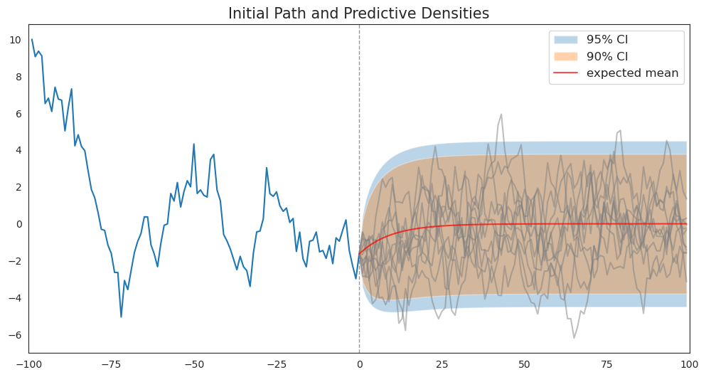
As functions of forecast horizon, the coverage intervals have shapes like those described in https://python.quantecon.org/perm_income_cons.html
19.3. Predictive Distributions of Path Properties#
Wecker [Wecker, 1979] proposed using simulation techniques to characterize predictive distribution of some statistics that are non-linear functions of
He called these functions “path properties” to contrast them with properties of single data points.
He studied two special prospective path properties of a given series
The first was time until the next turning point.
he defined a “turning point” to be the date of the second of two successive declines in
To examine this statistic, let
Then the random variable time until the next turning point is defined as the following stopping time with respect to
Wecker [Wecker, 1979] also studied the minimum value of
It is interesting to study yet another possible concept of a turning point.
Thus, let
Define a positive turning point today or tomorrow statistic as
This is designed to express the event
``after one or two decrease(s),
Following [Wecker, 1979], we can use simulations to calculate probabilities of
19.4. A Wecker-Like Algorithm#
The procedure consists of the following steps:
index a sample path by
for a given date
for each path
consider the sets
19.5. Using Simulations to Approximate a Posterior Distribution#
The next code cells use pymc to compute the time
Note that in defining the likelihood function, we choose to condition on the initial value
def draw_from_posterior(sample):
    """
    Draw a sample of size N from the posterior distribution.
    """

    AR1_model = pmc.Model()

    with AR1_model:

        # Start with priors
        rho = pmc.Uniform('rho',lower=-1.,upper=1.)  # Assume stable rho
        sigma = pmc.HalfNormal('sigma', sigma = np.sqrt(10))

        # Expected value of y at the next period (rho * y)
        yhat = rho * sample[:-1]

        # Likelihood of the actual realization.
        y_like = pmc.Normal('y_obs', mu=yhat, sigma=sigma, observed=sample[1:])

    with AR1_model:
        trace = pmc.sample(10000, tune=5000)

    # check condition
    with AR1_model:
        az.plot_trace(trace, figsize=(17, 6))

    rhos = trace.posterior.rho.values.flatten()
    sigmas = trace.posterior.sigma.values.flatten()

    post_sample = {
        'rho': rhos,
        'sigma': sigmas
    }

    return post_sample

post_samples = draw_from_posterior(initial_path)
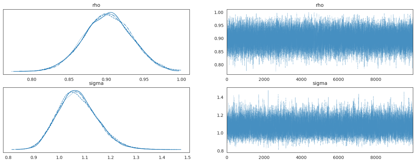
The graphs on the left portray posterior marginal distributions.
19.6. Calculating Sample Path Statistics#
Our next step is to prepare Python code to compute our sample path statistics.
# define statistics
def next_recession(omega):
    n = omega.shape[0] - 3
    z = np.zeros(n, dtype=int)

    for i in range(n):
        z[i] = int(omega[i] <= omega[i+1] and omega[i+1] > omega[i+2] and omega[i+2] > omega[i+3])

    if np.any(z) == False:
        return 500
    else:
        return np.where(z==1)[0][0] + 1

def minimum_value(omega):
    return min(omega[:8])

def severe_recession(omega):
    z = np.diff(omega)
    n = z.shape[0]

    sr = (z < -.02).astype(int)
    indices = np.where(sr == 1)[0]

    if len(indices) == 0:
        return T1
    else:
        return indices[0] + 1

def next_turning_point(omega):
    """
    Suppose that omega is of length 6

        y_{t-2}, y_{t-1}, y_{t}, y_{t+1}, y_{t+2}, y_{t+3}

    that is sufficient for determining the value of P/N
    """

    n = np.asarray(omega).shape[0] - 4
    T = np.zeros(n, dtype=int)

    for i in range(n):
        if ((omega[i] > omega[i+1]) and (omega[i+1] > omega[i+2]) and
            (omega[i+2] < omega[i+3]) and (omega[i+3] < omega[i+4])):
            T[i] = 1
        elif ((omega[i] < omega[i+1]) and (omega[i+1] < omega[i+2]) and
            (omega[i+2] > omega[i+3]) and (omega[i+3] > omega[i+4])):
            T[i] = -1

    up_turn = np.where(T == 1)[0][0] + 1 if (1 in T) == True else T1
    down_turn = np.where(T == -1)[0][0] + 1 if (-1 in T) == True else T1

    return up_turn, down_turn
19.7. Original Wecker Method#
Now we apply Wecker’s original method by simulating future paths and compute predictive distributions, conditioning on the true parameters associated with the data-generating model.
def plot_Wecker(initial_path, N, ax):
    """
    Plot the predictive distributions from "pure" Wecker's method.
    """
    # Store outcomes
    next_reces = np.zeros(N)
    severe_rec = np.zeros(N)
    min_vals = np.zeros(N)
    next_up_turn, next_down_turn = np.zeros(N), np.zeros(N)

    # Compute .9 confidence interval]
    y0 = initial_path[-1]
    center = np.array([rho**j * y0 for j in range(T1)])
    vars = np.array([sigma**2 * (1 - rho**(2 * j)) / (1 - rho**2) for j in range(T1)])
    y_bounds1_c95, y_bounds2_c95 = center + 1.96 * np.sqrt(vars), center - 1.96 * np.sqrt(vars)
    y_bounds1_c90, y_bounds2_c90 = center + 1.65 * np.sqrt(vars), center - 1.65 * np.sqrt(vars)

    # Plot
    ax[0, 0].set_title("Initial path and predictive densities", fontsize=15)
    ax[0, 0].plot(np.arange(-T0 + 1, 1), initial_path)
    ax[0, 0].set_xlim([-T0, T1])
    ax[0, 0].axvline(0, linestyle='--', alpha=.4, color='k', lw=1)

    # Plot 90% CI
    ax[0, 0].fill_between(np.arange(T1), y_bounds1_c95, y_bounds2_c95, alpha=.3)
    ax[0, 0].fill_between(np.arange(T1), y_bounds1_c90, y_bounds2_c90, alpha=.35)
    ax[0, 0].plot(np.arange(T1), center, color='red', alpha=.7)

    # Simulate future paths
    for n in range(N):
        sim_path = AR1_simulate(rho, sigma, initial_path[-1], T1)
        next_reces[n] = next_recession(np.hstack([initial_path[-3:-1], sim_path]))
        severe_rec[n] = severe_recession(sim_path)
        min_vals[n] = minimum_value(sim_path)
        next_up_turn[n], next_down_turn[n] = next_turning_point(sim_path)

        if n%(N/10) == 0:
            ax[0, 0].plot(np.arange(T1), sim_path, color='gray', alpha=.3, lw=1)

    # Return next_up_turn, next_down_turn
    sns.histplot(next_reces, kde=True, stat='density', ax=ax[0, 1], alpha=.8, label='True parameters')
    ax[0, 1].set_title("Predictive distribution of time until the next recession", fontsize=13)

    sns.histplot(severe_rec, kde=False, stat='density', ax=ax[1, 0], binwidth=0.9, alpha=.7, label='True parameters')
    ax[1, 0].set_title(r"Predictive distribution of stopping time of growth$<-2\%$", fontsize=13)

    sns.histplot(min_vals, kde=True, stat='density', ax=ax[1, 1], alpha=.8, label='True parameters')
    ax[1, 1].set_title("Predictive distribution of minimum value in the next 8 periods", fontsize=13)

    sns.histplot(next_up_turn, kde=True, stat='density', ax=ax[2, 0], alpha=.8, label='True parameters')
    ax[2, 0].set_title("Predictive distribution of time until the next positive turn", fontsize=13)

    sns.histplot(next_down_turn, kde=True, stat='density', ax=ax[2, 1], alpha=.8, label='True parameters')
    ax[2, 1].set_title("Predictive distribution of time until the next negative turn", fontsize=13)

fig, ax = plt.subplots(3, 2, figsize=(15,12))
plot_Wecker(initial_path, 1000, ax)
plt.show()
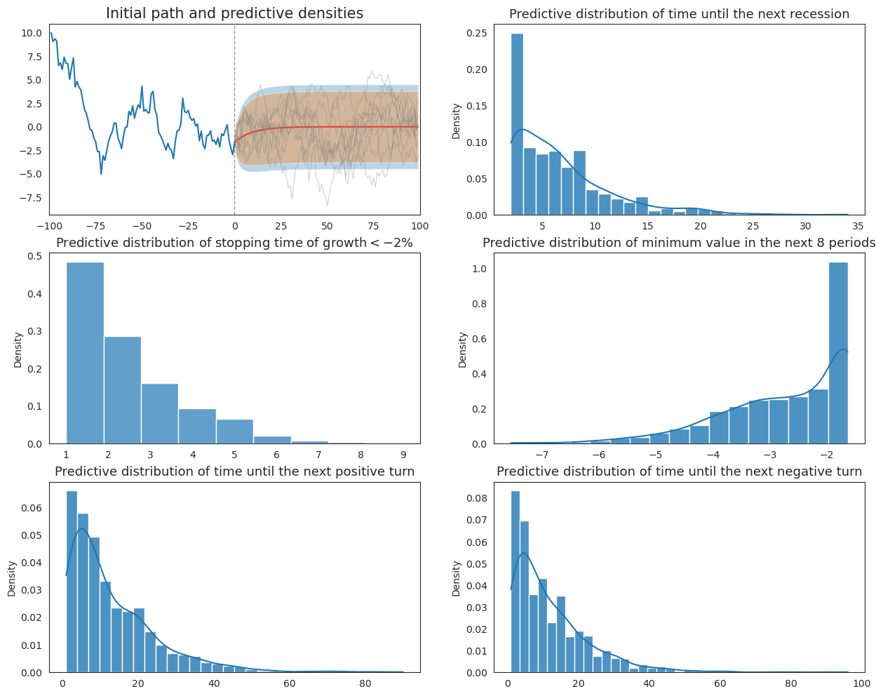
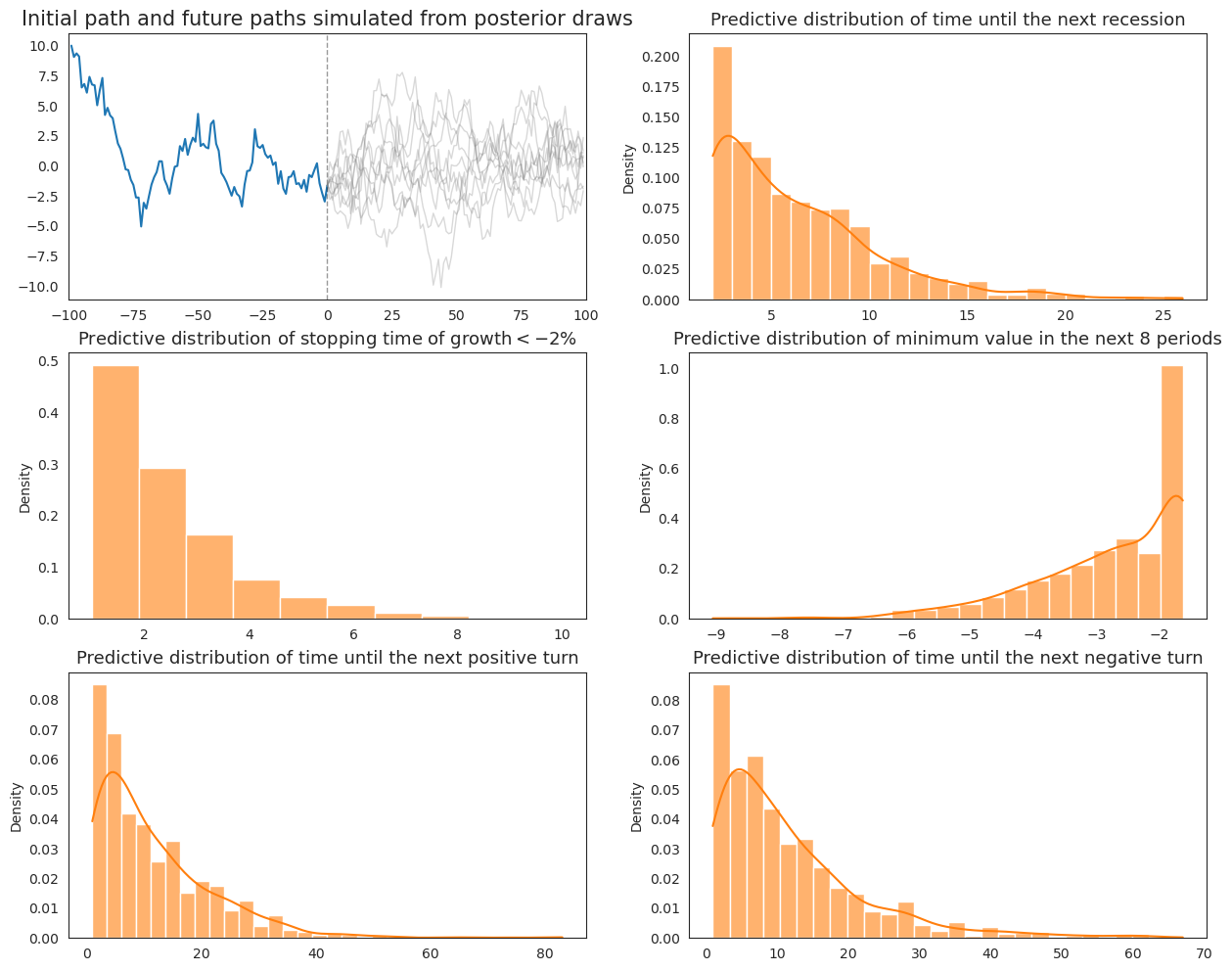
19.8. Extended Wecker Method#
Now we apply we apply our “extended” Wecker method based on predictive densities of
To approximate the intergration on the right side of (19.4), we repeatedly draw parameters from the joint posterior distribution each time we simulate a sequence of future values from model (19.1).
def plot_extended_Wecker(post_samples, initial_path, N, ax):
    """
    Plot the extended Wecker's predictive distribution
    """
    # Select a sample
    index = np.random.choice(np.arange(len(post_samples['rho'])), N + 1, replace=False)
    rho_sample = post_samples['rho'][index]
    sigma_sample = post_samples['sigma'][index]

    # Store outcomes
    next_reces = np.zeros(N)
    severe_rec = np.zeros(N)
    min_vals = np.zeros(N)
    next_up_turn, next_down_turn = np.zeros(N), np.zeros(N)

    # Plot
    ax[0, 0].set_title("Initial path and future paths simulated from posterior draws", fontsize=15)
    ax[0, 0].plot(np.arange(-T0 + 1, 1), initial_path)
    ax[0, 0].set_xlim([-T0, T1])
    ax[0, 0].axvline(0, linestyle='--', alpha=.4, color='k', lw=1)

    # Simulate future paths
    for n in range(N):
        sim_path = AR1_simulate(rho_sample[n], sigma_sample[n], initial_path[-1], T1)
        next_reces[n] = next_recession(np.hstack([initial_path[-3:-1], sim_path]))
        severe_rec[n] = severe_recession(sim_path)
        min_vals[n] = minimum_value(sim_path)
        next_up_turn[n], next_down_turn[n] = next_turning_point(sim_path)

        if n % (N / 10) == 0:
            ax[0, 0].plot(np.arange(T1), sim_path, color='gray', alpha=.3, lw=1)

    # Return next_up_turn, next_down_turn
    sns.histplot(next_reces, kde=True, stat='density', ax=ax[0, 1], alpha=.6, color=colors[1], label='Sampling from posterior')
    ax[0, 1].set_title("Predictive distribution of time until the next recession", fontsize=13)

    sns.histplot(severe_rec, kde=False, stat='density', ax=ax[1, 0], binwidth=.9, alpha=.6, color=colors[1], label='Sampling from posterior')
    ax[1, 0].set_title(r"Predictive distribution of stopping time of growth$<-2\%$", fontsize=13)

    sns.histplot(min_vals, kde=True, stat='density', ax=ax[1, 1], alpha=.6, color=colors[1], label='Sampling from posterior')
    ax[1, 1].set_title("Predictive distribution of minimum value in the next 8 periods", fontsize=13)

    sns.histplot(next_up_turn, kde=True, stat='density', ax=ax[2, 0], alpha=.6, color=colors[1], label='Sampling from posterior')
    ax[2, 0].set_title("Predictive distribution of time until the next positive turn", fontsize=13)

    sns.histplot(next_down_turn, kde=True, stat='density', ax=ax[2, 1], alpha=.6, color=colors[1], label='Sampling from posterior')
    ax[2, 1].set_title("Predictive distribution of time until the next negative turn", fontsize=13)

fig, ax = plt.subplots(3, 2, figsize=(15, 12))
plot_extended_Wecker(post_samples, initial_path, 1000, ax)
plt.show()
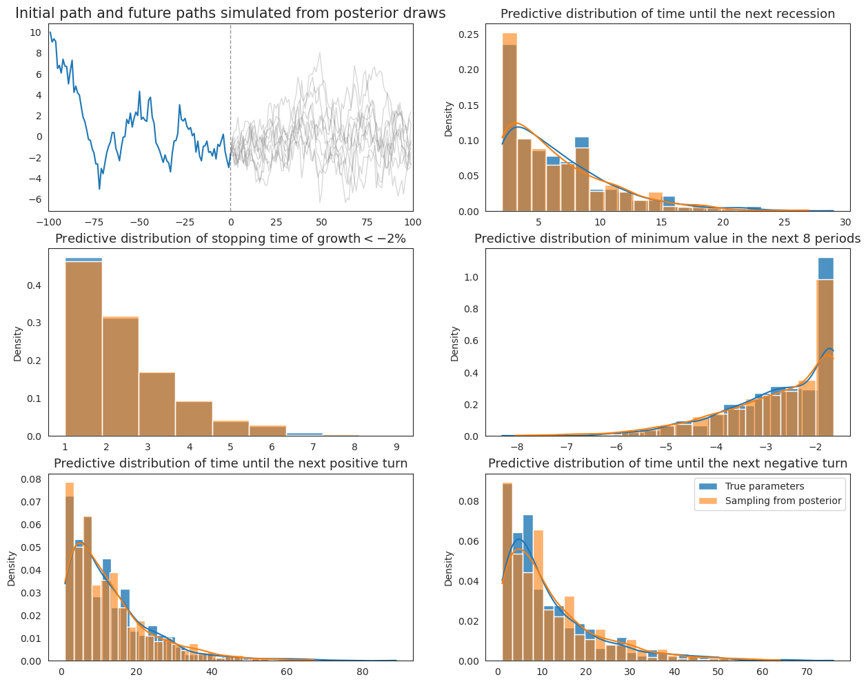
19.9. Comparison#
Finally, we plot both the original Wecker method and the extended method with parameter values drawn from the posterior together to compare the differences that emerge from pretending to know parameter values when they are actually uncertain.
fig, ax = plt.subplots(3, 2, figsize=(15,12))
plot_Wecker(initial_path, 1000, ax)
ax[0, 0].clear()
plot_extended_Wecker(post_samples, initial_path, 1000, ax)
plt.legend()
plt.show()