64. A Lake Model of Employment and Unemployment#
Contents
In addition to what’s in Anaconda, this lecture will need the following libraries:
!pip install quantecon
Show code cell output
Requirement already satisfied: quantecon in /home/runner/miniconda3/envs/quantecon/lib/python3.12/site-packages (0.8.1)
Requirement already satisfied: numba>=0.49.0 in /home/runner/miniconda3/envs/quantecon/lib/python3.12/site-packages (from quantecon) (0.60.0)
Requirement already satisfied: numpy>=1.17.0 in /home/runner/miniconda3/envs/quantecon/lib/python3.12/site-packages (from quantecon) (1.26.4)
Requirement already satisfied: requests in /home/runner/miniconda3/envs/quantecon/lib/python3.12/site-packages (from quantecon) (2.32.3)
Requirement already satisfied: scipy>=1.5.0 in /home/runner/miniconda3/envs/quantecon/lib/python3.12/site-packages (from quantecon) (1.13.1)
Requirement already satisfied: sympy in /home/runner/miniconda3/envs/quantecon/lib/python3.12/site-packages (from quantecon) (1.14.0)
Requirement already satisfied: llvmlite<0.44,>=0.43.0dev0 in /home/runner/miniconda3/envs/quantecon/lib/python3.12/site-packages (from numba>=0.49.0->quantecon) (0.43.0)
Requirement already satisfied: charset-normalizer<4,>=2 in /home/runner/miniconda3/envs/quantecon/lib/python3.12/site-packages (from requests->quantecon) (3.3.2)
Requirement already satisfied: idna<4,>=2.5 in /home/runner/miniconda3/envs/quantecon/lib/python3.12/site-packages (from requests->quantecon) (3.7)
Requirement already satisfied: urllib3<3,>=1.21.1 in /home/runner/miniconda3/envs/quantecon/lib/python3.12/site-packages (from requests->quantecon) (2.2.3)
Requirement already satisfied: certifi>=2017.4.17 in /home/runner/miniconda3/envs/quantecon/lib/python3.12/site-packages (from requests->quantecon) (2024.8.30)
Requirement already satisfied: mpmath<1.4,>=1.1.0 in /home/runner/miniconda3/envs/quantecon/lib/python3.12/site-packages (from sympy->quantecon) (1.3.0)
64.1. Overview#
This lecture describes what has come to be called a lake model.
The lake model is a basic tool for modeling unemployment.
It allows us to analyze
flows between unemployment and employment.
how these flows influence steady state employment and unemployment rates.
It is a good model for interpreting monthly labor department reports on gross and net jobs created and jobs destroyed.
The “lakes” in the model are the pools of employed and unemployed.
The “flows” between the lakes are caused by
firing and hiring
entry and exit from the labor force
For the first part of this lecture, the parameters governing transitions into and out of unemployment and employment are exogenous.
Later, we’ll determine some of these transition rates endogenously using the McCall search model.
We’ll also use some nifty concepts like ergodicity, which provides a fundamental link between cross-sectional and long run time series distributions.
These concepts will help us build an equilibrium model of ex-ante homogeneous workers whose different luck generates variations in their ex post experiences.
Let’s start with some imports:
import matplotlib.pyplot as plt
plt.rcParams["figure.figsize"] = (11, 5)  #set default figure size
import numpy as np
from quantecon import MarkovChain
from scipy.stats import norm
from scipy.optimize import brentq
from quantecon.distributions import BetaBinomial
from numba import jit
64.1.1. Prerequisites#
Before working through what follows, we recommend you read the lecture on finite Markov chains.
You will also need some basic linear algebra and probability.
64.2. The Model#
The economy is inhabited by a very large number of ex-ante identical workers.
The workers live forever, spending their lives moving between unemployment and employment.
Their rates of transition between employment and unemployment are governed by the following parameters:
The growth rate of the labor force evidently equals
64.2.1. Aggregate Variables#
We want to derive the dynamics of the following aggregates
We also want to know the values of the following objects
The employment rate
The unemployment rate
(Here and below, capital letters represent aggregates and lowercase letters represent rates)
64.2.2. Laws of Motion for Stock Variables#
We begin by constructing laws of motion for the aggregate variables
Of the mass of workers
of these,
Of the mass of workers
of these,
Therefore, the number of workers who will be employed at date
A similar analysis implies
The value
The total stock of workers
Letting
This law tells us how total employment and unemployment evolve over time.
64.2.3. Laws of Motion for Rates#
Now let’s derive the law of motion for rates.
To get these we can divide both sides of
Letting
we can also write this as
You can check that
This follows from the fact that the columns of
64.3. Implementation#
Let’s code up these equations.
To do this we’re going to use a class that we’ll call LakeModel.
This class will
store the primitives
compute and store the implied objects
provide methods to simulate dynamics of the stocks and rates
provide a method to compute the steady state vector
Please be careful because the implied objects
For example, if you would like to update a primitive like lm = LakeModel(α=0.03).
In the exercises, we show how to avoid this issue by using getter and setter methods.
class LakeModel:
    """
    Solves the lake model and computes dynamics of unemployment stocks and
    rates.

    Parameters:
    ------------
    λ : scalar
        The job finding rate for currently unemployed workers
    α : scalar
        The dismissal rate for currently employed workers
    b : scalar
        Entry rate into the labor force
    d : scalar
        Exit rate from the labor force

    """
    def __init__(self, λ=0.283, α=0.013, b=0.0124, d=0.00822):
        self.λ, self.α, self.b, self.d = λ, α, b, d

        λ, α, b, d = self.λ, self.α, self.b, self.d
        self.g = b - d
        self.A = np.array([[(1-d) * (1-λ) + b,      (1 - d) * α + b],
                           [        (1-d) * λ,      (1 - d) * (1 - α)]])

        self.A_hat = self.A / (1 + self.g)


    def rate_steady_state(self, tol=1e-6):
        """
        Finds the steady state of the system :math:`x_{t+1} = \hat A x_{t}`

        Returns
        --------
        xbar : steady state vector of employment and unemployment rates
        """
        x = np.array([self.A_hat[0, 1], self.A_hat[1, 0]])
        x /= x.sum()
        return x

    def simulate_stock_path(self, X0, T):
        """
        Simulates the sequence of Employment and Unemployment stocks

        Parameters
        ------------
        X0 : array
            Contains initial values (E0, U0)
        T : int
            Number of periods to simulate

        Returns
        ---------
        X : iterator
            Contains sequence of employment and unemployment stocks
        """

        X = np.atleast_1d(X0)  # Recast as array just in case
        for t in range(T):
            yield X
            X = self.A @ X

    def simulate_rate_path(self, x0, T):
        """
        Simulates the sequence of employment and unemployment rates

        Parameters
        ------------
        x0 : array
            Contains initial values (e0,u0)
        T : int
            Number of periods to simulate

        Returns
        ---------
        x : iterator
            Contains sequence of employment and unemployment rates

        """
        x = np.atleast_1d(x0)  # Recast as array just in case
        for t in range(T):
            yield x
            x = self.A_hat @ x
<>:30: SyntaxWarning: invalid escape sequence '\h'
<>:30: SyntaxWarning: invalid escape sequence '\h'
/tmp/ipykernel_6970/2374623047.py:30: SyntaxWarning: invalid escape sequence '\h'
  """
As explained, if we create an instance and update it by lm = LakeModel(α=0.03),
derived objects like
lm = LakeModel()
lm.α
0.013
lm.A
array([[0.72350626, 0.02529314],
       [0.28067374, 0.97888686]])
lm = LakeModel(α = 0.03)
lm.A
array([[0.72350626, 0.0421534 ],
       [0.28067374, 0.9620266 ]])
64.3.1. Aggregate Dynamics#
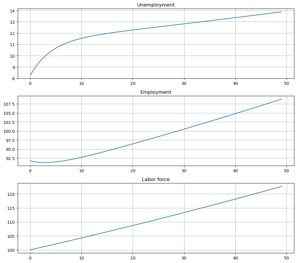
Let’s run a simulation under the default parameters (see above) starting from
lm = LakeModel()
N_0 = 150      # Population
e_0 = 0.92     # Initial employment rate
u_0 = 1 - e_0  # Initial unemployment rate
T = 50         # Simulation length

U_0 = u_0 * N_0
E_0 = e_0 * N_0

fig, axes = plt.subplots(3, 1, figsize=(10, 8))
X_0 = (U_0, E_0)
X_path = np.vstack(tuple(lm.simulate_stock_path(X_0, T)))

axes[0].plot(X_path[:, 0], lw=2)
axes[0].set_title('Unemployment')

axes[1].plot(X_path[:, 1], lw=2)
axes[1].set_title('Employment')

axes[2].plot(X_path.sum(1), lw=2)
axes[2].set_title('Labor force')

for ax in axes:
    ax.grid()

plt.tight_layout()
plt.show()
The aggregates
On the other hand, the vector of employment and unemployment rates
the components satisfy
This equation tells us that a steady state level
We also have
This is the case for our default parameters:
lm = LakeModel()
e, f = np.linalg.eigvals(lm.A_hat)
abs(e), abs(f)
(0.6953067378358462, 1.0)
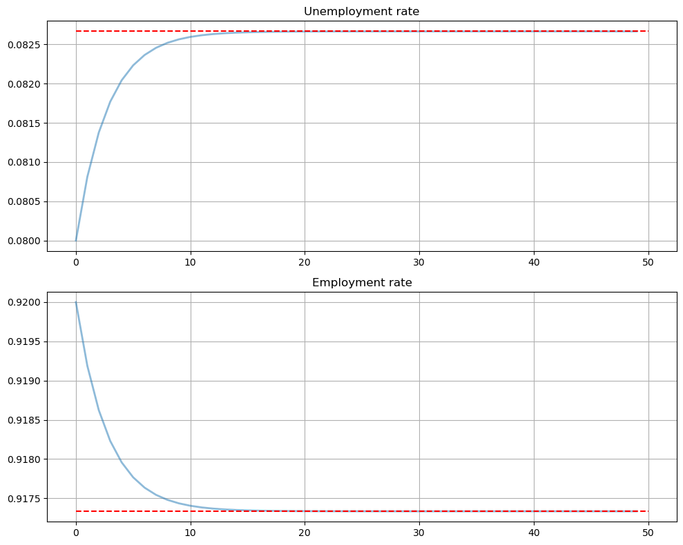
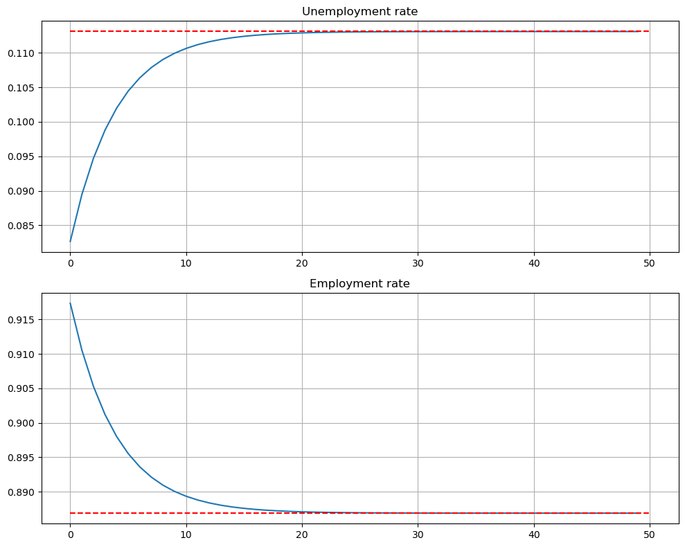
Let’s look at the convergence of the unemployment and employment rate to steady state levels (dashed red line)
lm = LakeModel()
e_0 = 0.92     # Initial employment rate
u_0 = 1 - e_0  # Initial unemployment rate
T = 50         # Simulation length

xbar = lm.rate_steady_state()

fig, axes = plt.subplots(2, 1, figsize=(10, 8))
x_0 = (u_0, e_0)
x_path = np.vstack(tuple(lm.simulate_rate_path(x_0, T)))

titles = ['Unemployment rate', 'Employment rate']

for i, title in enumerate(titles):
    axes[i].plot(x_path[:, i], lw=2, alpha=0.5)
    axes[i].hlines(xbar[i], 0, T, 'r', '--')
    axes[i].set_title(title)
    axes[i].grid()

plt.tight_layout()
plt.show()
64.4. Dynamics of an Individual Worker#
An individual worker’s employment dynamics are governed by a finite state Markov process.
The worker can be in one of two states:
Let’s start off under the assumption that
The associated transition matrix is then
Let
As usual, we regard it as a row vector.
We know from an earlier discussion that
We also know from the lecture on finite Markov chains
that if
The unique stationary distribution satisfies
Not surprisingly, probability mass on the unemployment state increases with the dismissal rate and falls with the job finding rate.
64.4.1. Ergodicity#
Let’s look at a typical lifetime of employment-unemployment spells.
We want to compute the average amounts of time an infinitely lived worker would spend employed and unemployed.
Let
and
(As usual,
These are the fraction of time a worker spends unemployed and employed, respectively, up until period
If
with probability one.
Inspection tells us that
Thus, the percentages of time that an infinitely lived worker spends employed and unemployed equal the fractions of workers employed and unemployed in the steady state distribution.
64.4.2. Convergence Rate#
How long does it take for time series sample averages to converge to cross-sectional averages?
We can use QuantEcon.py’s MarkovChain class to investigate this.
Let’s plot the path of the sample averages over 5,000 periods
lm = LakeModel(d=0, b=0)
T = 5000  # Simulation length

α, λ = lm.α, lm.λ

P = [[1 - λ,        λ],
    [    α,    1 - α]]

mc = MarkovChain(P)

xbar = lm.rate_steady_state()

fig, axes = plt.subplots(2, 1, figsize=(10, 8))
s_path = mc.simulate(T, init=1)
s_bar_e = s_path.cumsum() / range(1, T+1)
s_bar_u = 1 - s_bar_e

to_plot = [s_bar_u, s_bar_e]
titles = ['Percent of time unemployed', 'Percent of time employed']

for i, plot in enumerate(to_plot):
    axes[i].plot(plot, lw=2, alpha=0.5)
    axes[i].hlines(xbar[i], 0, T, 'r', '--')
    axes[i].set_title(titles[i])
    axes[i].grid()

plt.tight_layout()
plt.show()
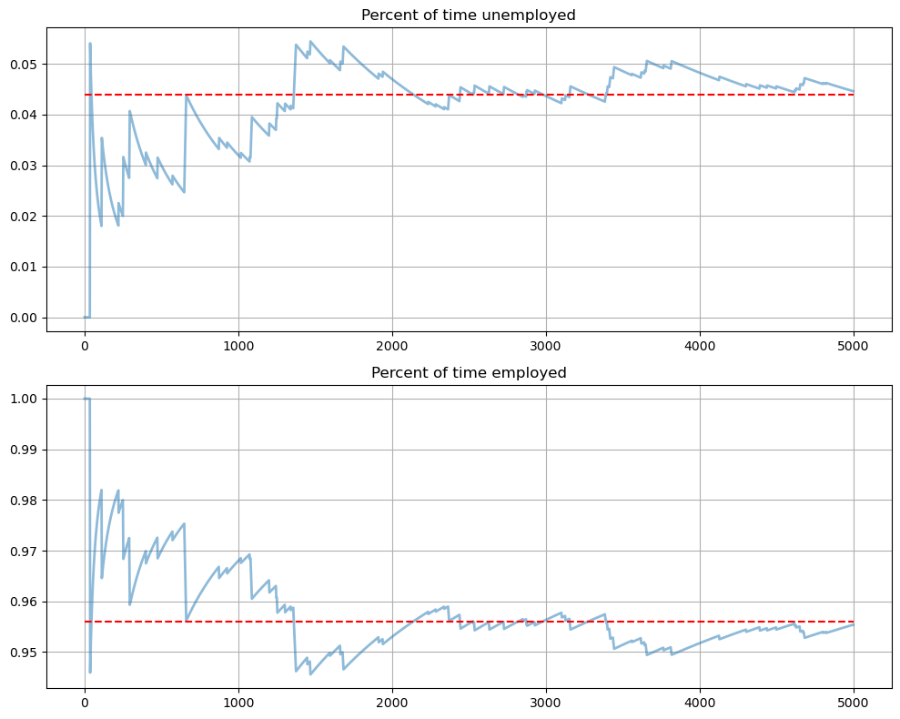
The stationary probabilities are given by the dashed red line.
In this case it takes much of the sample for these two objects to converge.
This is largely due to the high persistence in the Markov chain.
64.5. Endogenous Job Finding Rate#
We now make the hiring rate endogenous.
The transition rate from unemployment to employment will be determined by the McCall search model [McCall, 1970].
All details relevant to the following discussion can be found in our treatment of that model.
64.5.1. Reservation Wage#
The most important thing to remember about the model is that optimal decisions
are characterized by a reservation wage
If the wage offer
Otherwise, the worker rejects.
As we saw in our discussion of the model, the reservation wage depends on the wage offer distribution and the parameters
64.5.2. Linking the McCall Search Model to the Lake Model#
Suppose that all workers inside a lake model behave according to the McCall search model.
The exogenous probability of leaving employment remains
But their optimal decision rules determine the probability
This is now
64.5.3. Fiscal Policy#
We can use the McCall search version of the Lake Model to find an optimal level of unemployment insurance.
We assume that the government sets unemployment compensation
The government imposes a lump-sum tax
To attain a balanced budget at a steady state, taxes, the steady state unemployment rate
The lump-sum tax applies to everyone, including unemployed workers.
Thus, the post-tax income of an employed worker with wage
The post-tax income of an unemployed worker is
For each specification
This determines
For a given level of unemployment benefit
To evaluate alternative government tax-unemployment compensation pairs, we require a welfare criterion.
We use a steady state welfare criterion
where the notation
The wage offer distribution will be a discretized version of the lognormal distribution
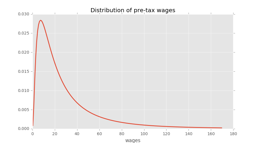
We take a period to be a month.
We set
Following [Davis et al., 2006], we set
64.5.4. Fiscal Policy Code#
We will make use of techniques from the McCall model lecture
The first piece of code implements value function iteration
# A default utility function

@jit
def u(c, σ):
    if c > 0:
        return (c**(1 - σ) - 1) / (1 - σ)
    else:
        return -10e6


class McCallModel:
    """
    Stores the parameters and functions associated with a given model.
    """

    def __init__(self,
                α=0.2,       # Job separation rate
                β=0.98,      # Discount rate
                γ=0.7,       # Job offer rate
                c=6.0,       # Unemployment compensation
                σ=2.0,       # Utility parameter
                w_vec=None,  # Possible wage values
                p_vec=None): # Probabilities over w_vec

        self.α, self.β, self.γ, self.c = α, β, γ, c
        self.σ = σ

        # Add a default wage vector and probabilities over the vector using
        # the beta-binomial distribution
        if w_vec is None:
            n = 60  # Number of possible outcomes for wage
            # Wages between 10 and 20
            self.w_vec = np.linspace(10, 20, n)
            a, b = 600, 400  # Shape parameters
            dist = BetaBinomial(n-1, a, b)
            self.p_vec = dist.pdf()
        else:
            self.w_vec = w_vec
            self.p_vec = p_vec

@jit
def _update_bellman(α, β, γ, c, σ, w_vec, p_vec, V, V_new, U):
    """
    A jitted function to update the Bellman equations.  Note that V_new is
    modified in place (i.e, modified by this function).  The new value of U
    is returned.

    """
    for w_idx, w in enumerate(w_vec):
        # w_idx indexes the vector of possible wages
        V_new[w_idx] = u(w, σ) + β * ((1 - α) * V[w_idx] + α * U)

    U_new = u(c, σ) + β * (1 - γ) * U + \
                    β * γ * np.sum(np.maximum(U, V) * p_vec)

    return U_new


def solve_mccall_model(mcm, tol=1e-5, max_iter=2000):
    """
    Iterates to convergence on the Bellman equations

    Parameters
    ----------
    mcm : an instance of McCallModel
    tol : float
        error tolerance
    max_iter : int
        the maximum number of iterations
    """

    V = np.ones(len(mcm.w_vec))  # Initial guess of V
    V_new = np.empty_like(V)     # To store updates to V
    U = 1                        # Initial guess of U
    i = 0
    error = tol + 1

    while error > tol and i < max_iter:
        U_new = _update_bellman(mcm.α, mcm.β, mcm.γ,
                mcm.c, mcm.σ, mcm.w_vec, mcm.p_vec, V, V_new, U)
        error_1 = np.max(np.abs(V_new - V))
        error_2 = np.abs(U_new - U)
        error = max(error_1, error_2)
        V[:] = V_new
        U = U_new
        i += 1

    return V, U
The second piece of code is used to complete the reservation wage:
def compute_reservation_wage(mcm, return_values=False):
    """
    Computes the reservation wage of an instance of the McCall model
    by finding the smallest w such that V(w) > U.

    If V(w) > U for all w, then the reservation wage w_bar is set to
    the lowest wage in mcm.w_vec.

    If v(w) < U for all w, then w_bar is set to np.inf.

    Parameters
    ----------
    mcm : an instance of McCallModel
    return_values : bool (optional, default=False)
        Return the value functions as well

    Returns
    -------
    w_bar : scalar
        The reservation wage

    """

    V, U = solve_mccall_model(mcm)
    w_idx = np.searchsorted(V - U, 0)

    if w_idx == len(V):
        w_bar = np.inf
    else:
        w_bar = mcm.w_vec[w_idx]

    if return_values == False:
        return w_bar
    else:
        return w_bar, V, U
Now let’s compute and plot welfare, employment, unemployment, and tax revenue as a function of the unemployment compensation rate
# Some global variables that will stay constant
α = 0.013
α_q = (1-(1-α)**3)   # Quarterly (α is monthly)
b = 0.0124
d = 0.00822
β = 0.98
γ = 1.0
σ = 2.0

# The default wage distribution --- a discretized lognormal
log_wage_mean, wage_grid_size, max_wage = 20, 200, 170
logw_dist = norm(np.log(log_wage_mean), 1)
w_vec = np.linspace(1e-8, max_wage, wage_grid_size + 1)
cdf = logw_dist.cdf(np.log(w_vec))
pdf = cdf[1:] - cdf[:-1]
p_vec = pdf / pdf.sum()
w_vec = (w_vec[1:] + w_vec[:-1]) / 2


def compute_optimal_quantities(c, τ):
    """
    Compute the reservation wage, job finding rate and value functions
    of the workers given c and τ.

    """

    mcm = McCallModel(α=α_q,
                    β=β,
                    γ=γ,
                    c=c-τ,          # Post tax compensation
                    σ=σ,
                    w_vec=w_vec-τ,  # Post tax wages
                    p_vec=p_vec)

    w_bar, V, U = compute_reservation_wage(mcm, return_values=True)
    λ = γ * np.sum(p_vec[w_vec - τ > w_bar])
    return w_bar, λ, V, U

def compute_steady_state_quantities(c, τ):
    """
    Compute the steady state unemployment rate given c and τ using optimal
    quantities from the McCall model and computing corresponding steady
    state quantities

    """
    w_bar, λ, V, U = compute_optimal_quantities(c, τ)

    # Compute steady state employment and unemployment rates
    lm = LakeModel(α=α_q, λ=λ, b=b, d=d)
    x = lm.rate_steady_state()
    u, e = x

    # Compute steady state welfare
    w = np.sum(V * p_vec * (w_vec - τ > w_bar)) / np.sum(p_vec * (w_vec -
            τ > w_bar))
    welfare = e * w + u * U

    return e, u, welfare


def find_balanced_budget_tax(c):
    """
    Find the tax level that will induce a balanced budget.

    """
    def steady_state_budget(t):
        e, u, w = compute_steady_state_quantities(c, t)
        return t - u * c

    τ = brentq(steady_state_budget, 0.0, 0.9 * c)
    return τ


# Levels of unemployment insurance we wish to study
c_vec = np.linspace(5, 140, 60)

tax_vec = []
unempl_vec = []
empl_vec = []
welfare_vec = []

for c in c_vec:
    t = find_balanced_budget_tax(c)
    e_rate, u_rate, welfare = compute_steady_state_quantities(c, t)
    tax_vec.append(t)
    unempl_vec.append(u_rate)
    empl_vec.append(e_rate)
    welfare_vec.append(welfare)

fig, axes = plt.subplots(2, 2, figsize=(12, 10))

plots = [unempl_vec, empl_vec, tax_vec, welfare_vec]
titles = ['Unemployment', 'Employment', 'Tax', 'Welfare']

for ax, plot, title in zip(axes.flatten(), plots, titles):
    ax.plot(c_vec, plot, lw=2, alpha=0.7)
    ax.set_title(title)
    ax.grid()

plt.tight_layout()
plt.show()
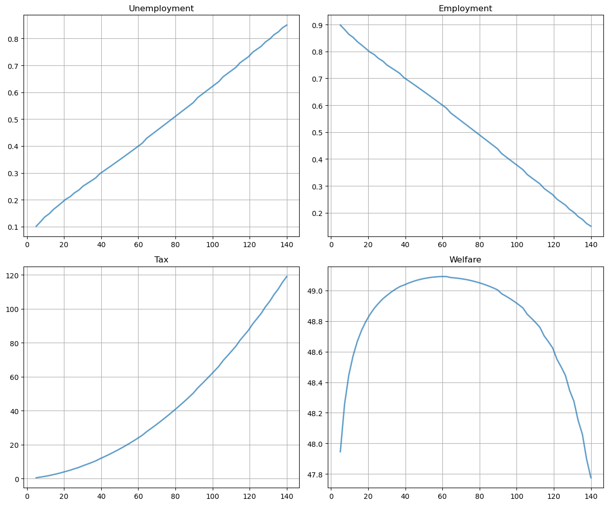
Welfare first increases and then decreases as unemployment benefits rise.
The level that maximizes steady state welfare is approximately 62.
64.6. Exercises#
Exercise 64.1
In the Lake Model, there is derived data such as
So, when a user alters these primitives, we need the derived data to update automatically.
(For example, if a user changes the value of
In the code above, we took care of this issue by creating new instances every time we wanted to change parameters.
That way the derived data is always matched to current parameter values.
However, we can use descriptors instead, so that derived data is updated whenever parameters are changed.
This is safer and means we don’t need to create a fresh instance for every new parameterization.
(On the other hand, the code becomes denser, which is why we don’t always use the descriptor approach in our lectures.)
In this exercise, your task is to arrange the LakeModel class by using descriptors and decorators such as @property.
(If you need to refresh your understanding of how these work, consult this lecture.)
Solution to Exercise 64.1
Here is one solution
class LakeModelModified:
    """
    Solves the lake model and computes dynamics of unemployment stocks and
    rates.

    Parameters:
    ------------
    λ : scalar
        The job finding rate for currently unemployed workers
    α : scalar
        The dismissal rate for currently employed workers
    b : scalar
        Entry rate into the labor force
    d : scalar
        Exit rate from the labor force

    """
    def __init__(self, λ=0.283, α=0.013, b=0.0124, d=0.00822):
        self._λ, self._α, self._b, self._d = λ, α, b, d
        self.compute_derived_values()

    def compute_derived_values(self):
        # Unpack names to simplify expression
        λ, α, b, d = self._λ, self._α, self._b, self._d

        self._g = b - d
        self._A = np.array([[(1-d) * (1-λ) + b,      (1 - d) * α + b],
                            [        (1-d) * λ,   (1 - d) * (1 - α)]])

        self._A_hat = self._A / (1 + self._g)

    @property
    def g(self):
        return self._g

    @property
    def A(self):
        return self._A

    @property
    def A_hat(self):
        return self._A_hat

    @property
    def λ(self):
        return self._λ

    @λ.setter
    def λ(self, new_value):
        self._λ = new_value
        self.compute_derived_values()

    @property
    def α(self):
        return self._α

    @α.setter
    def α(self, new_value):
        self._α = new_value
        self.compute_derived_values()

    @property
    def b(self):
        return self._b

    @b.setter
    def b(self, new_value):
        self._b = new_value
        self.compute_derived_values()

    @property
    def d(self):
        return self._d

    @d.setter
    def d(self, new_value):
        self._d = new_value
        self.compute_derived_values()


    def rate_steady_state(self, tol=1e-6):
        """
        Finds the steady state of the system :math:`x_{t+1} = \hat A x_{t}`

        Returns
        --------
        xbar : steady state vector of employment and unemployment rates
        """
        x = np.array([self.A_hat[0, 1], self.A_hat[1, 0]])
        x /= x.sum()
        return x

    def simulate_stock_path(self, X0, T):
        """
        Simulates the sequence of Employment and Unemployment stocks

        Parameters
        ------------
        X0 : array
            Contains initial values (E0, U0)
        T : int
            Number of periods to simulate

        Returns
        ---------
        X : iterator
            Contains sequence of employment and unemployment stocks
        """

        X = np.atleast_1d(X0)  # Recast as array just in case
        for t in range(T):
            yield X
            X = self.A @ X

    def simulate_rate_path(self, x0, T):
        """
        Simulates the sequence of employment and unemployment rates

        Parameters
        ------------
        x0 : array
            Contains initial values (e0,u0)
        T : int
            Number of periods to simulate

        Returns
        ---------
        x : iterator
            Contains sequence of employment and unemployment rates

        """
        x = np.atleast_1d(x0)  # Recast as array just in case
        for t in range(T):
            yield x
            x = self.A_hat @ x
<>:82: SyntaxWarning: invalid escape sequence '\h'
<>:82: SyntaxWarning: invalid escape sequence '\h'
/tmp/ipykernel_6970/2744789789.py:82: SyntaxWarning: invalid escape sequence '\h'
  """
Exercise 64.2
Consider an economy with an initial stock of workers
(The values for
Suppose that in response to new legislation the hiring rate reduces to
Plot the transition dynamics of the unemployment and employment stocks for 50 periods.
Plot the transition dynamics for the rates.
How long does the economy take to converge to its new steady state?
What is the new steady state level of employment?
Note
It may be easier to use the class created in exercise 1 to help with changing variables.
Solution to Exercise 64.2
We begin by constructing the class containing the default parameters and assigning the
steady state values to x0
lm = LakeModelModified()
x0 = lm.rate_steady_state()
print(f"Initial Steady State: {x0}")
Initial Steady State: [0.08266627 0.91733373]
Initialize the simulation values
N0 = 100
T = 50
New legislation changes
lm.λ = 0.2

xbar = lm.rate_steady_state()  # new steady state
X_path = np.vstack(tuple(lm.simulate_stock_path(x0 * N0, T)))
x_path = np.vstack(tuple(lm.simulate_rate_path(x0, T)))
print(f"New Steady State: {xbar}")
New Steady State: [0.11309295 0.88690705]
Now plot stocks
fig, axes = plt.subplots(3, 1, figsize=[10, 9])

axes[0].plot(X_path[:, 0])
axes[0].set_title('Unemployment')

axes[1].plot(X_path[:, 1])
axes[1].set_title('Employment')

axes[2].plot(X_path.sum(1))
axes[2].set_title('Labor force')

for ax in axes:
    ax.grid()

plt.tight_layout()
plt.show()
And how the rates evolve
fig, axes = plt.subplots(2, 1, figsize=(10, 8))

titles = ['Unemployment rate', 'Employment rate']

for i, title in enumerate(titles):
    axes[i].plot(x_path[:, i])
    axes[i].hlines(xbar[i], 0, T, 'r', '--')
    axes[i].set_title(title)
    axes[i].grid()

plt.tight_layout()
plt.show()
We see that it takes 20 periods for the economy to converge to its new steady state levels.
Exercise 64.3
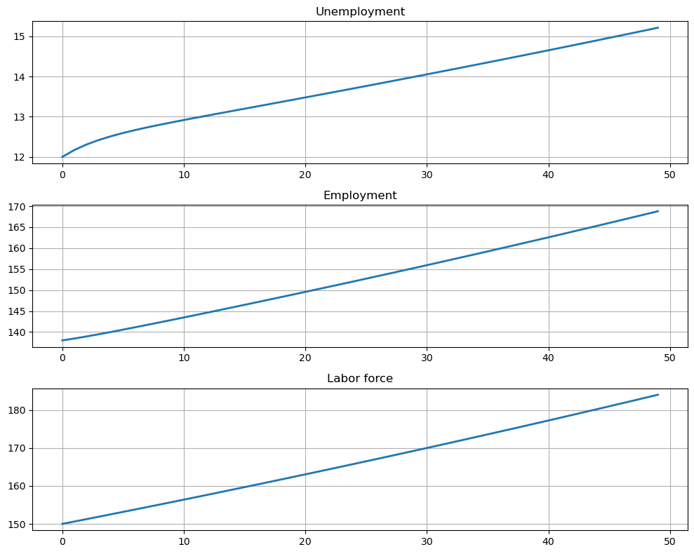
Consider an economy with an initial stock of workers
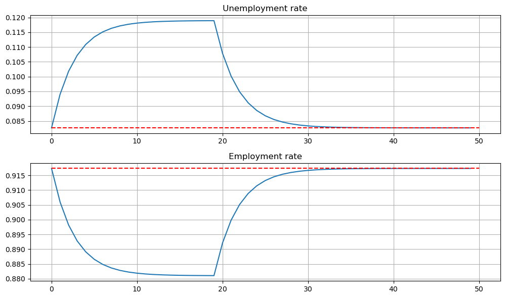
Suppose that for 20 periods the birth rate was temporarily high (
Plot the transition dynamics of the unemployment and employment stocks for 50 periods.
Plot the transition dynamics for the rates.
How long does the economy take to return to its original steady state?
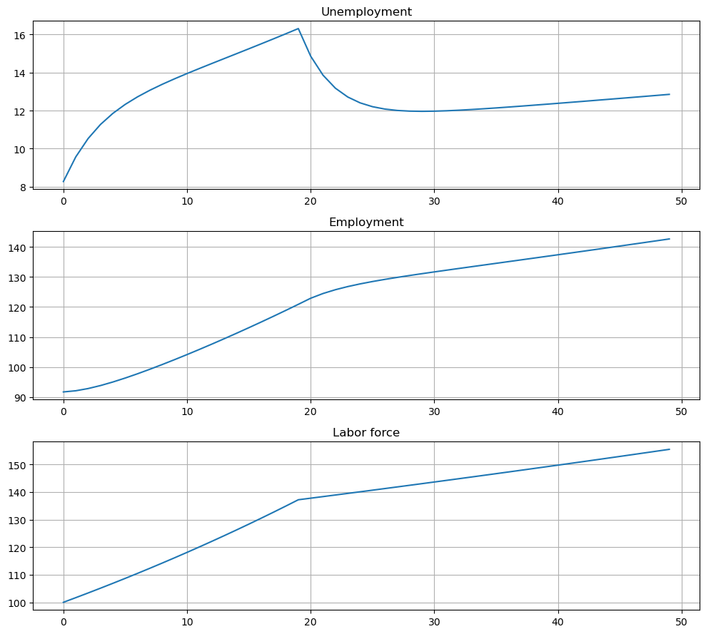
Solution to Exercise 64.3
This next exercise has the economy experiencing a boom in entrances to the labor market and then later returning to the original levels.
For 20 periods the economy has a new entry rate into the labor market.
Let’s start off at the baseline parameterization and record the steady state
lm = LakeModelModified()
x0 = lm.rate_steady_state()
Here are the other parameters:
b_hat = 0.025
T_hat = 20
Let’s increase
lm.b = b_hat
# Simulate stocks
X_path1 = np.vstack(tuple(lm.simulate_stock_path(x0 * N0, T_hat)))
# Simulate rates
x_path1 = np.vstack(tuple(lm.simulate_rate_path(x0, T_hat)))
Now we reset
lm.b = 0.0124
# Simulate stocks
X_path2 = np.vstack(tuple(lm.simulate_stock_path(X_path1[-1, :2], T-T_hat+1)))
# Simulate rates
x_path2 = np.vstack(tuple(lm.simulate_rate_path(x_path1[-1, :2], T-T_hat+1)))
Finally, we combine these two paths and plot
# note [1:] to avoid doubling period 20
x_path = np.vstack([x_path1, x_path2[1:]])
X_path = np.vstack([X_path1, X_path2[1:]])

fig, axes = plt.subplots(3, 1, figsize=[10, 9])

axes[0].plot(X_path[:, 0])
axes[0].set_title('Unemployment')

axes[1].plot(X_path[:, 1])
axes[1].set_title('Employment')

axes[2].plot(X_path.sum(1))
axes[2].set_title('Labor force')

for ax in axes:
    ax.grid()

plt.tight_layout()
plt.show()
And the rates
fig, axes = plt.subplots(2, 1, figsize=[10, 6])

titles = ['Unemployment rate', 'Employment rate']

for i, title in enumerate(titles):
    axes[i].plot(x_path[:, i])
    axes[i].hlines(x0[i], 0, T, 'r', '--')
    axes[i].set_title(title)
    axes[i].grid()

plt.tight_layout()
plt.show()