70. Asset Pricing: Finite State Models#
Contents
“A little knowledge of geometric series goes a long way” – Robert E. Lucas, Jr.
“Asset pricing is all about covariances” – Lars Peter Hansen
In addition to what’s in Anaconda, this lecture will need the following libraries:
!pip install quantecon
Show code cell output
Requirement already satisfied: quantecon in /home/runner/miniconda3/envs/quantecon/lib/python3.12/site-packages (0.8.1)
Requirement already satisfied: numba>=0.49.0 in /home/runner/miniconda3/envs/quantecon/lib/python3.12/site-packages (from quantecon) (0.60.0)
Requirement already satisfied: numpy>=1.17.0 in /home/runner/miniconda3/envs/quantecon/lib/python3.12/site-packages (from quantecon) (1.26.4)
Requirement already satisfied: requests in /home/runner/miniconda3/envs/quantecon/lib/python3.12/site-packages (from quantecon) (2.32.3)
Requirement already satisfied: scipy>=1.5.0 in /home/runner/miniconda3/envs/quantecon/lib/python3.12/site-packages (from quantecon) (1.13.1)
Requirement already satisfied: sympy in /home/runner/miniconda3/envs/quantecon/lib/python3.12/site-packages (from quantecon) (1.14.0)
Requirement already satisfied: llvmlite<0.44,>=0.43.0dev0 in /home/runner/miniconda3/envs/quantecon/lib/python3.12/site-packages (from numba>=0.49.0->quantecon) (0.43.0)
Requirement already satisfied: charset-normalizer<4,>=2 in /home/runner/miniconda3/envs/quantecon/lib/python3.12/site-packages (from requests->quantecon) (3.3.2)
Requirement already satisfied: idna<4,>=2.5 in /home/runner/miniconda3/envs/quantecon/lib/python3.12/site-packages (from requests->quantecon) (3.7)
Requirement already satisfied: urllib3<3,>=1.21.1 in /home/runner/miniconda3/envs/quantecon/lib/python3.12/site-packages (from requests->quantecon) (2.2.3)
Requirement already satisfied: certifi>=2017.4.17 in /home/runner/miniconda3/envs/quantecon/lib/python3.12/site-packages (from requests->quantecon) (2024.8.30)
Requirement already satisfied: mpmath<1.4,>=1.1.0 in /home/runner/miniconda3/envs/quantecon/lib/python3.12/site-packages (from sympy->quantecon) (1.3.0)
70.1. Overview#
An asset is a claim on one or more future payoffs.
The spot price of an asset depends primarily on
the anticipated income stream
attitudes about risk
rates of time preference
In this lecture, we consider some standard pricing models and dividend stream specifications.
We study how prices and dividend-price ratios respond in these different scenarios.
We also look at creating and pricing derivative assets that repackage income streams.
Key tools for the lecture are
Markov processses
formulas for predicting future values of functions of a Markov state
a formula for predicting the discounted sum of future values of a Markov state
Let’s start with some imports:
import matplotlib.pyplot as plt
plt.rcParams["figure.figsize"] = (11, 5)  #set default figure size
import numpy as np
import quantecon as qe
from numpy.linalg import eigvals, solve
70.2. Pricing Models#
Let
A time-
A time-
Let’s look at some equations that we expect to hold for prices of assets under ex-dividend contracts (we will consider cum-dividend pricing in the exercises).
70.2.1. Risk-Neutral Pricing#
Our first scenario is risk-neutral pricing.
Let
The basic risk-neutral asset pricing equation for pricing one unit of an ex-dividend asset is
This is a simple “cost equals expected benefit” relationship.
Here
More precisely,
70.2.2. Pricing with Random Discount Factor#
What happens if for some reason traders discount payouts differently depending on the state of the world?
Michael Harrison and David Kreps [Harrison and Kreps, 1979] and Lars Peter Hansen and Scott Richard [Hansen and Richard, 1987] showed that in quite general settings the price of an ex-dividend asset obeys
for some stochastic discount factor
Here the fixed discount factor
How anticipated future payoffs are evaluated now depends on statistical properties of
The stochastic discount factor can be specified to capture the idea that assets that tend to have good payoffs in bad states of the world are valued more highly than other assets whose payoffs don’t behave that way.
This is because such assets pay well when funds are more urgently wanted.
We give examples of how the stochastic discount factor has been modeled below.
70.2.3. Asset Pricing and Covariances#
Recall that, from the definition of a conditional covariance
If we apply this definition to the asset pricing equation (70.2) we obtain
It is useful to regard equation (70.4) as a generalization of equation (70.1)
In equation (70.1), the stochastic discount factor
In equation (70.1), the covariance term
In equation (70.1),
When
Equation (70.4) asserts that the covariance of the stochastic discount factor with the one period payout
We give examples of some models of stochastic discount factors that have been proposed later in this lecture and also in a later lecture.
70.2.4. The Price-Dividend Ratio#
Aside from prices, another quantity of interest is the price-dividend ratio
Let’s write down an expression that this ratio should satisfy.
We can divide both sides of (70.2) by
Below we’ll discuss the implication of this equation.
70.3. Prices in the Risk-Neutral Case#
What can we say about price dynamics on the basis of the models described above?
The answer to this question depends on
the process we specify for dividends
the stochastic discount factor and how it correlates with dividends
For now we’ll study the risk-neutral case in which the stochastic discount factor is constant.
We’ll focus on how an asset price depends on a dividend process.
70.3.1. Example 1: Constant Dividends#
The simplest case is risk-neutral price of a constant, non-random dividend stream
Removing the expectation from (70.1) and iterating forward gives
If
This is the equilibrium price in the constant dividend case.
Indeed, simple algebra shows that setting
70.3.2. Example 2: Dividends with Deterministic Growth Paths#
Consider a growing, non-random dividend process
While prices are not usually constant when dividends grow over time, a price dividend-ratio can be.
If we guess this, substituting
Since
The price is then
If, in this example, we take
This is called the Gordon formula.
70.3.3. Example 3: Markov Growth, Risk-Neutral Pricing#
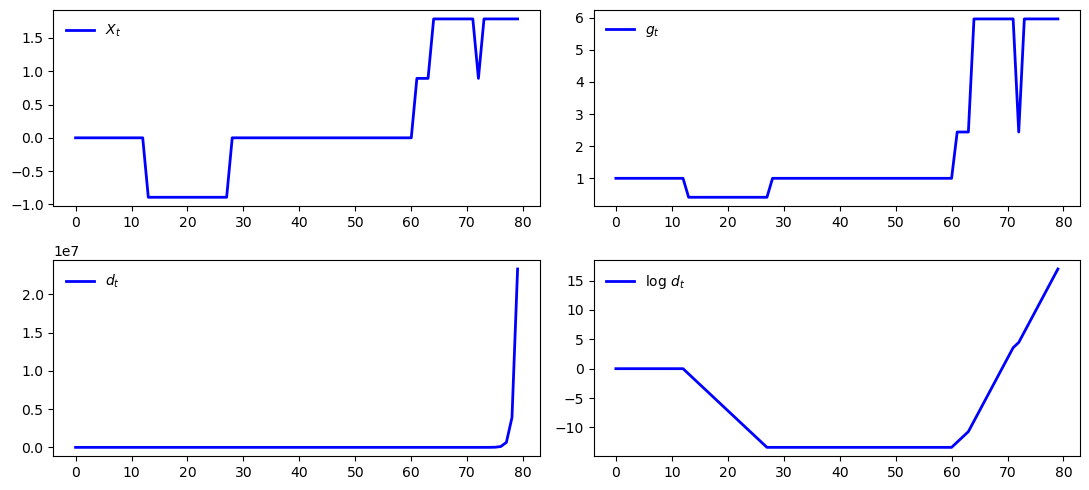
Next, we consider a dividend process
The stochastic growth factor
where
You can think of
(For a refresher on notation and theory for finite Markov chains see this lecture)
The next figure shows a simulation, where
n = 7
mc = qe.tauchen(n, 0.96, 0.25)
sim_length = 80

x_series = mc.simulate(sim_length, init=np.median(mc.state_values))
g_series = np.exp(x_series)
d_series = np.cumprod(g_series) # Assumes d_0 = 1

series = [x_series, g_series, d_series, np.log(d_series)]
labels = ['$X_t$', '$g_t$', '$d_t$', r'$\log \, d_t$']

fig, axes = plt.subplots(2, 2)
for ax, s, label in zip(axes.flatten(), series, labels):
    ax.plot(s, 'b-', lw=2, label=label)
    ax.legend(loc='upper left', frameon=False)
plt.tight_layout()
plt.show()
70.3.3.1. Pricing Formula#
To obtain asset prices in this setting, let’s adapt our analysis from the case of deterministic growth.
In that case, we found that
This encourages us to guess that, in the current case,
We seek a function
We can substitute this guess into (70.5) to get
If we condition on
or
Suppose that there are
We can then think of (70.8) as
Here
When does equation (70.9) have a unique solution?
From the Neumann series lemma and Gelfand’s formula, equation (70.9) has a unique solution when
Thus, we require that the eigenvalues of
The solution is then
70.3.4. Code#
Let’s calculate and plot the price-dividend ratio at some parameters.
As before, we’ll generate
Here’s the code, including a test of the spectral radius condition
n = 25  # Size of state space
β = 0.9
mc = qe.tauchen(n, 0.96, 0.02)

K = mc.P * np.exp(mc.state_values)

warning_message = "Spectral radius condition fails"
assert np.max(np.abs(eigvals(K))) < 1 / β,  warning_message

I = np.identity(n)
v = solve(I - β * K, β * K @ np.ones(n))

fig, ax = plt.subplots()
ax.plot(mc.state_values, v, 'g-o', lw=2, alpha=0.7, label='$v$')
ax.set_ylabel("price-dividend ratio")
ax.set_xlabel("state")
ax.legend(loc='upper left')
plt.show()
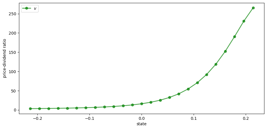
Why does the price-dividend ratio increase with the state?
The reason is that this Markov process is positively correlated, so high current states suggest high future states.
Moreover, dividend growth is increasing in the state.
The anticipation of high future dividend growth leads to a high price-dividend ratio.
70.4. Risk Aversion and Asset Prices#
Now let’s turn to the case where agents are risk averse.
We’ll price several distinct assets, including
An endowment stream
A consol (a type of bond issued by the UK government in the 19th century)
Call options on a consol
70.4.1. Pricing a Lucas Tree#
Let’s start with a version of the celebrated asset pricing model of Robert E. Lucas, Jr. [Lucas, 1978].
Lucas considered an abstract pure exchange economy with these features:
a single non-storable consumption good
a Markov process that governs the total amount of the consumption good available each period
a single tree that each period yields fruit that equals the total amount of consumption available to the economy
a competitive market in shares in the tree that entitles their owners to corresponding shares of the dividend stream, i.e., the fruit stream, yielded by the tree
a representative consumer who in a competitive equilibrium
consumes the economy’s entire endowment each period
owns 100 percent of the shares in the tree
As in [Lucas, 1978], we suppose that the stochastic discount factor takes the form
where
(A derivation of this expression is given in a later lecture)
Assume the existence of an endowment that follows growth process (70.7).
The asset being priced is a claim on the endowment process, i.e., the Lucas tree described above.
Following [Lucas, 1978], we suppose that in equilibrium the representative consumer’s consumption equals the aggregate endowment, so that
For utility, we’ll assume the constant relative risk aversion (CRRA) specification
When
Inserting the CRRA specification into (70.11) and using
Substituting this into (70.5) gives the price-dividend ratio formula
Conditioning on
If we let
then we can rewrite equation (70.14) in vector form as
Assuming that the spectral radius of
We will define a function tree_price to compute
class AssetPriceModel:
    """
    A class that stores the primitives of the asset pricing model.

    Parameters
    ----------
    β : scalar, float
        Discount factor
    mc : MarkovChain
        Contains the transition matrix and set of state values for the state
        process
    γ : scalar(float)
        Coefficient of risk aversion
    g : callable
        The function mapping states to growth rates

    """
    def __init__(self, β=0.96, mc=None, γ=2.0, g=np.exp):
        self.β, self.γ = β, γ
        self.g = g

        # A default process for the Markov chain
        if mc is None:
            self.ρ = 0.9
            self.σ = 0.02
            self.mc = qe.tauchen(n, self.ρ, self.σ)
        else:
            self.mc = mc

        self.n = self.mc.P.shape[0]

    def test_stability(self, Q):
        """
        Stability test for a given matrix Q.
        """
        sr = np.max(np.abs(eigvals(Q)))
        if not sr < 1 / self.β:
            msg = f"Spectral radius condition failed with radius = {sr}"
            raise ValueError(msg)


def tree_price(ap):
    """
    Computes the price-dividend ratio of the Lucas tree.

    Parameters
    ----------
    ap: AssetPriceModel
        An instance of AssetPriceModel containing primitives

    Returns
    -------
    v : array_like(float)
        Lucas tree price-dividend ratio

    """
    # Simplify names, set up matrices
    β, γ, P, y = ap.β, ap.γ, ap.mc.P, ap.mc.state_values
    J = P * ap.g(y)**(1 - γ)

    # Make sure that a unique solution exists
    ap.test_stability(J)

    # Compute v
    I = np.identity(ap.n)
    Ones = np.ones(ap.n)
    v = solve(I - β * J, β * J @ Ones)

    return v
Here’s a plot of
γs = [1.2, 1.4, 1.6, 1.8, 2.0]
ap = AssetPriceModel()
states = ap.mc.state_values

fig, ax = plt.subplots()

for γ in γs:
    ap.γ = γ
    v = tree_price(ap)
    ax.plot(states, v, lw=2, alpha=0.6, label=rf"$\gamma = {γ}$")

ax.set_title('Price-dividend ratio as a function of the state')
ax.set_ylabel("price-dividend ratio")
ax.set_xlabel("state")
ax.legend(loc='upper right')
plt.show()
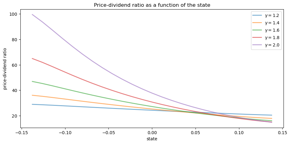
Notice that
This is because, with a positively correlated state process, higher states indicate higher future consumption growth.
With the stochastic discount factor (70.13), higher growth decreases the discount factor, lowering the weight placed on future dividends.
70.4.1.1. Special Cases#
In the special case
Recalling that
Thus, with log preferences, the price-dividend ratio for a Lucas tree is constant.
Alternatively, if
This is as expected, since
70.4.2. A Risk-Free Consol#
Consider the same pure exchange representative agent economy.
A risk-free consol promises to pay a constant amount
Recycling notation, let
An ex-coupon claim to the consol entitles an owner at the end of period
the right to sell the claim for
The price satisfies (70.2) with
With the stochastic discount factor (70.13), this becomes
Guessing a solution of the form
Letting
The above is implemented in the function consol_price.
def consol_price(ap, ζ):
    """
    Computes price of a consol bond with payoff ζ

    Parameters
    ----------
    ap: AssetPriceModel
        An instance of AssetPriceModel containing primitives

    ζ : scalar(float)
        Coupon of the console

    Returns
    -------
    p : array_like(float)
        Console bond prices

    """
    # Simplify names, set up matrices
    β, γ, P, y = ap.β, ap.γ, ap.mc.P, ap.mc.state_values
    M = P * ap.g(y)**(- γ)

    # Make sure that a unique solution exists
    ap.test_stability(M)

    # Compute price
    I = np.identity(ap.n)
    Ones = np.ones(ap.n)
    p = solve(I - β * M, β * ζ * M @ Ones)

    return p
70.4.3. Pricing an Option to Purchase the Consol#
Let’s now price options of various maturities.
We’ll study an option that gives the owner the right to purchase a consol at a price
70.4.3.1. An Infinite Horizon Call Option#
We want to price an infinite horizon option to purchase a consol at a price
The option entitles the owner at the beginning of a period either
to purchase the bond at price
not to exercise the option to purchase the asset now but to retain the right to exercise it later
Thus, the owner either exercises the option now or chooses not to exercise and wait until next period.
This is termed an infinite-horizon call option with strike price
The owner of the option is entitled to purchase the consol at price
The fundamentals of the economy are identical with the one above, including the stochastic discount factor and the process for consumption.
Let
Recalling that
The first term on the right is the value of waiting, while the second is the value of exercising now.
We can also write this as
With
To solve (70.19), form an operator
Start at some initial
We can find the solution with the following function call_option
def call_option(ap, ζ, p_s, ϵ=1e-7):
    """
    Computes price of a call option on a consol bond.

    Parameters
    ----------
    ap: AssetPriceModel
        An instance of AssetPriceModel containing primitives

    ζ : scalar(float)
        Coupon of the console

    p_s : scalar(float)
        Strike price

    ϵ : scalar(float), optional(default=1e-8)
        Tolerance for infinite horizon problem

    Returns
    -------
    w : array_like(float)
        Infinite horizon call option prices

    """
    # Simplify names, set up matrices
    β, γ, P, y = ap.β, ap.γ, ap.mc.P, ap.mc.state_values
    M = P * ap.g(y)**(- γ)

    # Make sure that a unique consol price exists
    ap.test_stability(M)

    # Compute option price
    p = consol_price(ap, ζ)
    w = np.zeros(ap.n)
    error = ϵ + 1
    while error > ϵ:
        # Maximize across columns
        w_new = np.maximum(β * M @ w, p - p_s)
        # Find maximal difference of each component and update
        error = np.amax(np.abs(w - w_new))
        w = w_new

    return w
Here’s a plot of
ap = AssetPriceModel(β=0.9)
ζ = 1.0
strike_price = 40

x = ap.mc.state_values
p = consol_price(ap, ζ)
w = call_option(ap, ζ, strike_price)

fig, ax = plt.subplots()
ax.plot(x, p, 'b-', lw=2, label='consol price')
ax.plot(x, w, 'g-', lw=2, label='value of call option')
ax.set_xlabel("state")
ax.legend(loc='upper right')
plt.show()
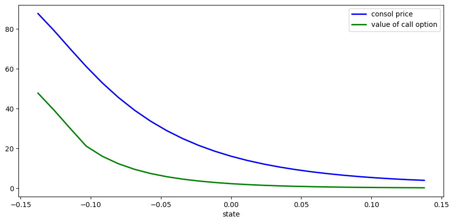
In high values of the Markov growth state, the value of the option is close to zero.
This is despite the facts that the Markov chain is irreducible and that low states — where the consol prices are high — will be visited recurrently.
The reason for low valuations in high Markov growth states is that
70.4.4. Risk-Free Rates#
Let’s look at risk-free interest rates over different periods.
70.4.4.1. The One-period Risk-free Interest Rate#
As before, the stochastic discount factor is
It follows that the reciprocal
We can write this as
where the
70.4.4.2. Other Terms#
Let
Then
70.5. Exercises#
Exercise 70.1
In the lecture, we considered ex-dividend assets.
A cum-dividend asset is a claim to the stream
Following (70.1), find the risk-neutral asset pricing equation for one unit of a cum-dividend asset.
With a constant, non-random dividend stream
With a growing, non-random dividend process
Solution to Exercise 70.1
For a cum-dividend asset, the basic risk-neutral asset pricing equation is
With constant dividends, the equilibrium price is
With a growing, non-random dividend process, the equilibrium price is
Exercise 70.2
Consider the following primitives
n = 5  # Size of State Space
P = np.full((n, n), 0.0125)
P[range(n), range(n)] += 1 - P.sum(1)
# State values of the Markov chain
s = np.array([0.95, 0.975, 1.0, 1.025, 1.05])
γ = 2.0
β = 0.94
Let
Compute the price of the Lucas tree.
Do the same for
the price of the risk-free consol when
the call option on the consol when
Solution to Exercise 70.2
First, let’s enter the parameters:
n = 5
P = np.full((n, n), 0.0125)
P[range(n), range(n)] += 1 - P.sum(1)
s = np.array([0.95, 0.975, 1.0, 1.025, 1.05])  # State values
mc = qe.MarkovChain(P, state_values=s)

γ = 2.0
β = 0.94
ζ = 1.0
p_s = 150.0
Next, we’ll create an instance of AssetPriceModel to feed into the
functions
apm = AssetPriceModel(β=β, mc=mc, γ=γ, g=lambda x: x)
Now we just need to call the relevant functions on the data:
tree_price(apm)
array([29.47401578, 21.93570661, 17.57142236, 14.72515002, 12.72221763])
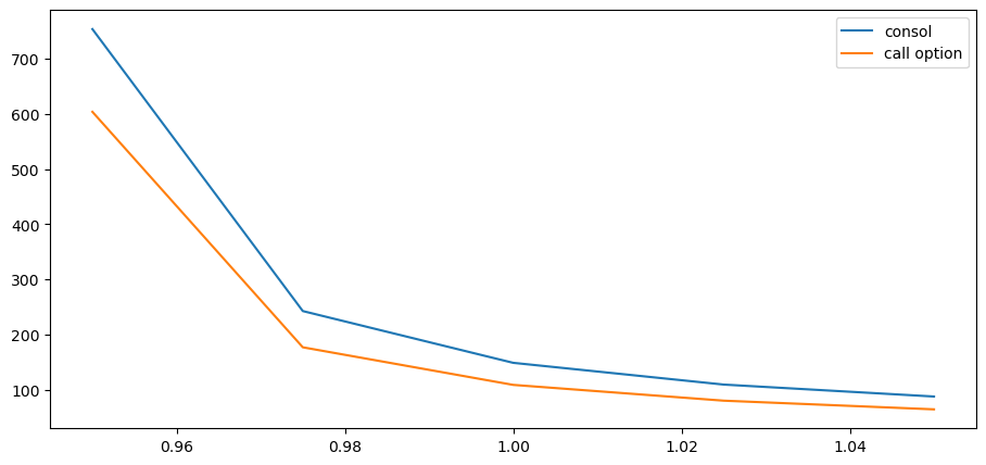
consol_price(apm, ζ)
array([753.87100476, 242.55144082, 148.67554548, 109.25108965,
        87.56860139])
call_option(apm, ζ, p_s)
array([603.87100476, 176.8393343 , 108.67734499,  80.05179254,
        64.30843748])
Let’s show the last two functions as a plot
fig, ax = plt.subplots()
ax.plot(s, consol_price(apm, ζ), label='consol')
ax.plot(s, call_option(apm, ζ, p_s), label='call option')
ax.legend()
plt.show()
Exercise 70.3
Let’s consider finite horizon call options, which are more common than infinite horizon ones.
Finite horizon options obey functional equations closely related to (70.18).
A
If we view today as date zero, a
The option expires at time
Thus, for
It obeys
where
We can express this as a sequence of nonlinear vector equations
Write a function that computes
Compute the value of the option with k = 5 and k = 25 using parameter values as in Exercise 70.1.
Is one higher than the other? Can you give intuition?
Solution to Exercise 70.3
Here’s a suitable function:
def finite_horizon_call_option(ap, ζ, p_s, k):
    """
    Computes k period option value.
    """
    # Simplify names, set up matrices
    β, γ, P, y = ap.β, ap.γ, ap.mc.P, ap.mc.state_values
    M = P * ap.g(y)**(- γ)

    # Make sure that a unique solution exists
    ap.test_stability(M)


    # Compute option price
    p = consol_price(ap, ζ)
    w = np.zeros(ap.n)
    for i in range(k):
        # Maximize across columns
        w = np.maximum(β * M @ w, p - p_s)

    return w
Now let’s compute the option values at k=5 and k=25
fig, ax = plt.subplots()
for k in [5, 25]:
    w = finite_horizon_call_option(apm, ζ, p_s, k)
    ax.plot(s, w, label=rf'$k = {k}$')
ax.legend()
plt.show()
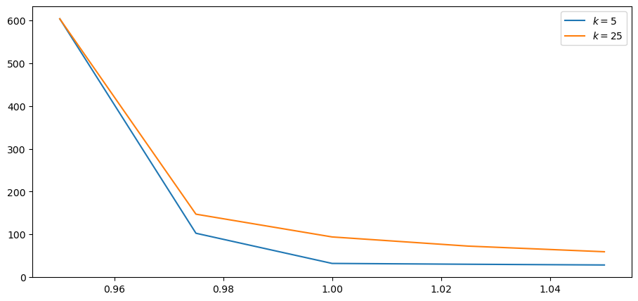
Not surprisingly, options with larger
This is because an owner has a longer horizon over which the option can be exercised.