12. Multivariate Normal Distribution #

Contents

Multivariate Normal Distribution

12.1. Overview #

This lecture describes a workhorse in probability theory, statistics, and economics, namely, the multivariate normal distribution.

In this lecture, you will learn formulas for

the joint distribution of a random vector $x$ of length $N$
marginal distributions for all subvectors of $x$
conditional distributions for subvectors of $x$ conditional on other subvectors of $x$

We will use the multivariate normal distribution to formulate some useful models:

a factor analytic model of an intelligence quotient, i.e., IQ
a factor analytic model of two independent inherent abilities, say, mathematical and verbal.
a more general factor analytic model
Principal Components Analysis (PCA) as an approximation to a factor analytic model
time series generated by linear stochastic difference equations
optimal linear filtering theory

12.2. The Multivariate Normal Distribution #

This lecture defines a Python class MultivariateNormal to be used to generate marginal and conditional distributions associated with a multivariate normal distribution.

For a multivariate normal distribution it is very convenient that

conditional expectations equal linear least squares projections
conditional distributions are characterized by multivariate linear regressions

We apply our Python class to some examples.

We use the following imports:

import matplotlib.pyplot as plt
plt.rcParams["figure.figsize"] = (11, 5)  #set default figure size
import numpy as np
from numba import jit
import statsmodels.api as sm

Assume that an $N \times 1$ random vector $z$ has a multivariate normal probability density.

This means that the probability density takes the form

f (z; μ, Σ) = {(2 π)}^{- (\frac{N}{2})} det {(Σ)}^{- \frac{1}{2}} \exp (- .5 {(z - μ)}^{'} Σ^{- 1} (z - μ))

where $μ = E z$ is the mean of the random vector $z$ and $Σ = E (z - μ) {(z - μ)}^{'}$ is the covariance matrix of $z$ .

The covariance matrix $Σ$ is symmetric and positive definite.

@jit
def f(z, μ, Σ):
    """
    The density function of multivariate normal distribution.

    Parameters
    ---------------
    z: ndarray(float, dim=2)
        random vector, N by 1
    μ: ndarray(float, dim=1 or 2)
        the mean of z, N by 1
    Σ: ndarray(float, dim=2)
        the covarianece matrix of z, N by 1
    """

    z = np.atleast_2d(z)
    μ = np.atleast_2d(μ)
    Σ = np.atleast_2d(Σ)

    N = z.size

    temp1 = np.linalg.det(Σ) ** (-1/2)
    temp2 = np.exp(-.5 * (z - μ).T @ np.linalg.inv(Σ) @ (z - μ))

    return (2 * np.pi) ** (-N/2) * temp1 * temp2

For some integer $k \in {1, \dots, N - 1}$ , partition $z$ as

\begin{array}{r} z = [\begin{array}{c} z_{1} \\ z_{2} \end{array}], \end{array}

where $z_{1}$ is an $(N - k) \times 1$ vector and $z_{2}$ is a $k \times 1$ vector.

Let

\begin{array}{r} μ = [\begin{array}{c} μ_{1} \\ μ_{2} \end{array}], Σ = [\begin{array}{cc} Σ_{11} & Σ_{12} \\ Σ_{21} & Σ_{22} \end{array}] \end{array}

be corresponding partitions of $μ$ and $Σ$ .

The marginal distribution of $z_{1}$ is

multivariate normal with mean $μ_{1}$ and covariance matrix $Σ_{11}$ .

The marginal distribution of $z_{2}$ is

multivariate normal with mean $μ_{2}$ and covariance matrix $Σ_{22}$ .

The distribution of $z_{1}$ conditional on $z_{2}$ is

multivariate normal with mean

{\hat{μ}}_{1} = μ_{1} + β (z_{2} - μ_{2})

and covariance matrix

{\hat{Σ}}_{11} = Σ_{11} - Σ_{12} Σ_{22}^{- 1} Σ_{21} = Σ_{11} - β Σ_{22} β^{'}

where

β = Σ_{12} Σ_{22}^{- 1}

is an $(N - k) \times k$ matrix of population regression coefficients of the $(N - k) \times 1$ random vector $z_{1} - μ_{1}$ on the $k \times 1$ random vector $z_{2} - μ_{2}$ .

The following class constructs a multivariate normal distribution instance with two methods.

a method partition computes $β$ , taking $k$ as an input
a method cond_dist computes either the distribution of $z_{1}$ conditional on $z_{2}$ or the distribution of $z_{2}$ conditional on $z_{1}$

class MultivariateNormal:
    """
    Class of multivariate normal distribution.

    Parameters
    ----------
    μ: ndarray(float, dim=1)
        the mean of z, N by 1
    Σ: ndarray(float, dim=2)
        the covarianece matrix of z, N by 1

    Arguments
    ---------
    μ, Σ:
        see parameters
    μs: list(ndarray(float, dim=1))
        list of mean vectors μ1 and μ2 in order
    Σs: list(list(ndarray(float, dim=2)))
        2 dimensional list of covariance matrices
        Σ11, Σ12, Σ21, Σ22 in order
    βs: list(ndarray(float, dim=1))
        list of regression coefficients β1 and β2 in order
    """

    def __init__(self, μ, Σ):
        "initialization"
        self.μ = np.array(μ)
        self.Σ = np.atleast_2d(Σ)

    def partition(self, k):
        """
        Given k, partition the random vector z into a size k vector z1
        and a size N-k vector z2. Partition the mean vector μ into
        μ1 and μ2, and the covariance matrix Σ into Σ11, Σ12, Σ21, Σ22
        correspondingly. Compute the regression coefficients β1 and β2
        using the partitioned arrays.
        """
        μ = self.μ
        Σ = self.Σ

        self.μs = [μ[:k], μ[k:]]
        self.Σs = [[Σ[:k, :k], Σ[:k, k:]],
                   [Σ[k:, :k], Σ[k:, k:]]]

        self.βs = [self.Σs[0][1] @ np.linalg.inv(self.Σs[1][1]),
                   self.Σs[1][0] @ np.linalg.inv(self.Σs[0][0])]

    def cond_dist(self, ind, z):
        """
        Compute the conditional distribution of z1 given z2, or reversely.
        Argument ind determines whether we compute the conditional
        distribution of z1 (ind=0) or z2 (ind=1).

        Returns
        ---------
        μ_hat: ndarray(float, ndim=1)
            The conditional mean of z1 or z2.
        Σ_hat: ndarray(float, ndim=2)
            The conditional covariance matrix of z1 or z2.
        """
        β = self.βs[ind]
        μs = self.μs
        Σs = self.Σs

        μ_hat = μs[ind] + β @ (z - μs[1-ind])
        Σ_hat = Σs[ind][ind] - β @ Σs[1-ind][1-ind] @ β.T

        return μ_hat, Σ_hat

Let’s put this code to work on a suite of examples.

We begin with a simple bivariate example; after that we’ll turn to a trivariate example.

We’ll compute population moments of some conditional distributions using our MultivariateNormal class.

For fun we’ll also compute sample analogs of the associated population regressions by generating simulations and then computing linear least squares regressions.

We’ll compare those linear least squares regressions for the simulated data to their population counterparts.

12.3. Bivariate Example #

We start with a bivariate normal distribution pinned down by

\begin{array}{r} μ = [\begin{array}{c} .5 \\ 1.0 \end{array}], Σ = [\begin{array}{cc} 1 & .5 \\ .5 & 1 \end{array}] \end{array}

μ = np.array([.5, 1.])
Σ = np.array([[1., .5], [.5 ,1.]])

# construction of the multivariate normal instance
multi_normal = MultivariateNormal(μ, Σ)

k = 1 # choose partition

# partition and compute regression coefficients
multi_normal.partition(k)
multi_normal.βs[0],multi_normal.βs[1]

(array([[0.5]]), array([[0.5]]))

Let’s illustrate the fact that you can regress anything on anything else.

We have computed everything we need to compute two regression lines, one of $z_{2}$ on $z_{1}$ , the other of $z_{1}$ on $z_{2}$ .

We’ll represent these regressions as

z_{1} = a_{1} + b_{1} z_{2} + ϵ_{1}

and

z_{2} = a_{2} + b_{2} z_{1} + ϵ_{2}

where we have the population least squares orthogonality conditions

E ϵ_{1} z_{2} = 0

and

E ϵ_{2} z_{1} = 0

Let’s compute $a_{1}, a_{2}, b_{1}, b_{2}$ .

beta = multi_normal.βs

a1 = μ[0] - beta[0]*μ[1]
b1 = beta[0]

a2 = μ[1] - beta[1]*μ[0]
b2 = beta[1]

Let’s print out the intercepts and slopes.

For the regression of $z_{1}$ on $z_{2}$ we have

print ("a1 = ", a1)
print ("b1 = ", b1)

a1 =  [[0.]]
b1 =  [[0.5]]

For the regression of $z_{2}$ on $z_{1}$ we have

print ("a2 = ", a2)
print ("b2 = ", b2)

a2 =  [[0.75]]
b2 =  [[0.5]]

Now let’s plot the two regression lines and stare at them.

z2 = np.linspace(-4,4,100)


a1 = np.squeeze(a1)
b1 = np.squeeze(b1)

a2 = np.squeeze(a2)
b2 = np.squeeze(b2)

z1  = b1*z2 + a1


z1h = z2/b2 - a2/b2


fig = plt.figure(figsize=(12,12))
ax = fig.add_subplot(1, 1, 1)
ax.set(xlim=(-4, 4), ylim=(-4, 4))
ax.spines['left'].set_position('center')
ax.spines['bottom'].set_position('zero')
ax.spines['right'].set_color('none')
ax.spines['top'].set_color('none')
ax.xaxis.set_ticks_position('bottom')
ax.yaxis.set_ticks_position('left')
plt.ylabel('$z_1$', loc = 'top')
plt.xlabel('$z_2$,', loc = 'right')
plt.title('two regressions')
plt.plot(z2,z1, 'r', label = "$z_1$ on $z_2$")
plt.plot(z2,z1h, 'b', label = "$z_2$ on $z_1$")
plt.legend()
plt.show()

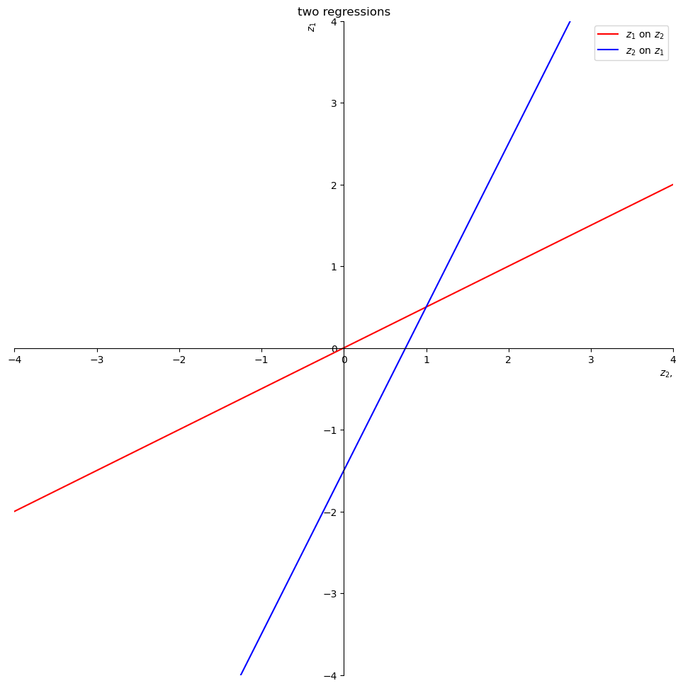
_images/160dc67acc7ad5fd43bb2c120b40a471f6a800a427bda1c66a762f689cc754cc.png

The red line is the expectation of $z_{1}$ conditional on $z_{2}$ .

The intercept and slope of the red line are

print("a1 = ", a1)
print("b1 = ", b1)

a1 =  0.0
b1 =  0.5

The blue line is the expectation of $z_{2}$ conditional on $z_{1}$ .

The intercept and slope of the blue line are

print("-a2/b2 = ", - a2/b2)
print("1/b2 = ", 1/b2)

-a2/b2 =  -1.5
1/b2 =  2.0

We can use these regression lines or our code to compute conditional expectations.

Let’s compute the mean and variance of the distribution of $z_{2}$ conditional on $z_{1} = 5$ .

After that we’ll reverse what are on the left and right sides of the regression.

# compute the cond. dist. of z1
ind = 1
z1 = np.array([5.]) # given z1

μ2_hat, Σ2_hat = multi_normal.cond_dist(ind, z1)
print('μ2_hat, Σ2_hat = ', μ2_hat, Σ2_hat)

μ2_hat, Σ2_hat =  [3.25] [[0.75]]

Now let’s compute the mean and variance of the distribution of $z_{1}$ conditional on $z_{2} = 5$ .

# compute the cond. dist. of z1
ind = 0
z2 = np.array([5.]) # given z2

μ1_hat, Σ1_hat = multi_normal.cond_dist(ind, z2)
print('μ1_hat, Σ1_hat = ', μ1_hat, Σ1_hat)

μ1_hat, Σ1_hat =  [2.5] [[0.75]]

Let’s compare the preceding population mean and variance with outcomes from drawing a large sample and then regressing $z_{1} - μ_{1}$ on $z_{2} - μ_{2}$ .

We know that

E z_{1} | z_{2} = (μ_{1} - β μ_{2}) + β z_{2}

which can be arranged to

z_{1} - μ_{1} = β (z_{2} - μ_{2}) + ϵ,

We anticipate that for larger and larger sample sizes, estimated OLS coefficients will converge to $β$ and the estimated variance of $ϵ$ will converge to ${\hat{Σ}}_{1}$ .

n = 1_000_000 # sample size

# simulate multivariate normal random vectors
data = np.random.multivariate_normal(μ, Σ, size=n)
z1_data = data[:, 0]
z2_data = data[:, 1]

# OLS regression
μ1, μ2 = multi_normal.μs
results = sm.OLS(z1_data - μ1, z2_data - μ2).fit()

Let’s compare the preceding population $β$ with the OLS sample estimate on $z_{2} - μ_{2}$

multi_normal.βs[0], results.params

(array([[0.5]]), array([0.50023899]))

Let’s compare our population ${\hat{Σ}}_{1}$ with the degrees-of-freedom adjusted estimate of the variance of $ϵ$

Σ1_hat, results.resid @ results.resid.T / (n - 1)

(array([[0.75]]), 0.7501698706292744)

Lastly, let’s compute the estimate of $\hat{E z_{1} | z_{2}}$ and compare it with ${\hat{μ}}_{1}$

μ1_hat, results.predict(z2 - μ2) + μ1

(array([2.5]), array([2.50095595]))

Thus, in each case, for our very large sample size, the sample analogues closely approximate their population counterparts.

A Law of Large Numbers explains why sample analogues approximate population objects.

12.4. Trivariate Example #

Let’s apply our code to a trivariate example.

We’ll specify the mean vector and the covariance matrix as follows.

μ = np.random.random(3)
C = np.random.random((3, 3))
Σ = C @ C.T # positive semi-definite

multi_normal = MultivariateNormal(μ, Σ)

μ, Σ

(array([0.70655948, 0.41884944, 0.57227581]),
 array([[0.28459369, 0.26256164, 0.38978302],
        [0.26256164, 0.51197677, 0.36294358],
        [0.38978302, 0.36294358, 1.53707536]]))

k = 1
multi_normal.partition(k)

Let’s compute the distribution of $z_{1}$ conditional on $z_{2} = [\begin{matrix} 2 \\ 5 \end{matrix}]$ .

ind = 0
z2 = np.array([2., 5.])

μ1_hat, Σ1_hat = multi_normal.cond_dist(ind, z2)

n = 1_000_000
data = np.random.multivariate_normal(μ, Σ, size=n)
z1_data = data[:, :k]
z2_data = data[:, k:]

μ1, μ2 = multi_normal.μs
results = sm.OLS(z1_data - μ1, z2_data - μ2).fit()

As above, we compare population and sample regression coefficients, the conditional covariance matrix, and the conditional mean vector in that order.

multi_normal.βs[0], results.params

(array([[0.40003092, 0.15912971]]), array([0.40048621, 0.1585142 ]))

Σ1_hat, results.resid @ results.resid.T / (n - 1)

(array([[0.11753485]]), 0.1178189244754668)

μ1_hat, results.predict(z2 - μ2) + μ1

(array([2.04365108]), array([2.04164564]))

Once again, sample analogues do a good job of approximating their populations counterparts.

12.5. One Dimensional Intelligence (IQ)#

Let’s move closer to a real-life example, namely, inferring a one-dimensional measure of intelligence called IQ from a list of test scores.

The $i$ th test score $y_{i}$ equals the sum of an unknown scalar IQ $θ$ and a random variable $w_{i}$ .

y_{i} = θ + σ_{y} w_{i}, i = 1, \dots, n

The distribution of IQ’s for a cross-section of people is a normal random variable described by

θ = μ_{θ} + σ_{θ} w_{n + 1} .

We assume that the noises ${w_{i}}_{i = 1}^{N}$ in the test scores are IID and not correlated with IQ.

We also assume that ${w_{i}}_{i = 1}^{n + 1}$ are i.i.d. standard normal:

\begin{array}{r} w = [\begin{array}{c} w_{1} \\ w_{2} \\ ⋮ \\ w_{n} \\ w_{n + 1} \end{array}] \sim N (0, I_{n + 1}) \end{array}

The following system describes the $(n + 1) \times 1$ random vector $X$ that interests us:

\begin{array}{r} X = [\begin{array}{c} y_{1} \\ y_{2} \\ ⋮ \\ y_{n} \\ θ \end{array}] = [\begin{array}{c} μ_{θ} \\ μ_{θ} \\ ⋮ \\ μ_{θ} \\ μ_{θ} \end{array}] + [\begin{array}{ccccc} σ_{y} & 0 & \dots & 0 & σ_{θ} \\ 0 & σ_{y} & \dots & 0 & σ_{θ} \\ ⋮ & ⋮ & ⋱ & ⋮ & ⋮ \\ 0 & 0 & \dots & σ_{y} & σ_{θ} \\ 0 & 0 & \dots & 0 & σ_{θ} \end{array}] [\begin{array}{c} w_{1} \\ w_{2} \\ ⋮ \\ w_{n} \\ w_{n + 1} \end{array}], \end{array}

or equivalently,

X = μ_{θ} 1_{n + 1} + D w

where $X = [\begin{matrix} y \\ θ \end{matrix}]$ , $1_{n + 1}$ is a vector of $1$ s of size $n + 1$ , and $D$ is an $n + 1$ by $n + 1$ matrix.

Let’s define a Python function that constructs the mean $μ$ and covariance matrix $Σ$ of the random vector $X$ that we know is governed by a multivariate normal distribution.

As arguments, the function takes the number of tests $n$ , the mean $μ_{θ}$ and the standard deviation $σ_{θ}$ of the IQ distribution, and the standard deviation of the randomness in test scores $σ_{y}$ .

def construct_moments_IQ(n, μθ, σθ, σy):

    μ_IQ = np.full(n+1, μθ)

    D_IQ = np.zeros((n+1, n+1))
    D_IQ[range(n), range(n)] = σy
    D_IQ[:, n] = σθ

    Σ_IQ = D_IQ @ D_IQ.T

    return μ_IQ, Σ_IQ, D_IQ

Now let’s consider a specific instance of this model.

Assume we have recorded $50$ test scores and we know that $μ_{θ} = 100$ , $σ_{θ} = 10$ , and $σ_{y} = 10$ .

We can compute the mean vector and covariance matrix of $X$ easily with our construct_moments_IQ function as follows.

n = 50
μθ, σθ, σy = 100., 10., 10.

μ_IQ, Σ_IQ, D_IQ = construct_moments_IQ(n, μθ, σθ, σy)
μ_IQ, Σ_IQ, D_IQ

(array([100., 100., 100., 100., 100., 100., 100., 100., 100., 100., 100.,
        100., 100., 100., 100., 100., 100., 100., 100., 100., 100., 100.,
        100., 100., 100., 100., 100., 100., 100., 100., 100., 100., 100.,
        100., 100., 100., 100., 100., 100., 100., 100., 100., 100., 100.,
        100., 100., 100., 100., 100., 100., 100.]),
 array([[200., 100., 100., ..., 100., 100., 100.],
        [100., 200., 100., ..., 100., 100., 100.],
        [100., 100., 200., ..., 100., 100., 100.],
        ...,
        [100., 100., 100., ..., 200., 100., 100.],
        [100., 100., 100., ..., 100., 200., 100.],
        [100., 100., 100., ..., 100., 100., 100.]]),
 array([[10.,  0.,  0., ...,  0.,  0., 10.],
        [ 0., 10.,  0., ...,  0.,  0., 10.],
        [ 0.,  0., 10., ...,  0.,  0., 10.],
        ...,
        [ 0.,  0.,  0., ..., 10.,  0., 10.],
        [ 0.,  0.,  0., ...,  0., 10., 10.],
        [ 0.,  0.,  0., ...,  0.,  0., 10.]]))

We can now use our MultivariateNormal class to construct an instance, then partition the mean vector and covariance matrix as we wish.

We want to regress IQ, the random variable $θ$ (what we don’t know), on the vector $y$ of test scores (what we do know).

We choose k=n so that $z_{1} = y$ and $z_{2} = θ$ .

multi_normal_IQ = MultivariateNormal(μ_IQ, Σ_IQ)

k = n
multi_normal_IQ.partition(k)

Using the generator multivariate_normal, we can make one draw of the random vector from our distribution and then compute the distribution of $θ$ conditional on our test scores.

Let’s do that and then print out some pertinent quantities.

x = np.random.multivariate_normal(μ_IQ, Σ_IQ)
y = x[:-1] # test scores
θ = x[-1]  # IQ

# the true value
θ

98.40800901560205

The method cond_dist takes test scores $y$ as input and returns the conditional normal distribution of the IQ $θ$ .

In the following code, ind sets the variables on the right side of the regression.

Given the way we have defined the vector $X$ , we want to set ind=1 in order to make $θ$ the left side variable in the population regression.

ind = 1
multi_normal_IQ.cond_dist(ind, y)

(array([97.35083863]), array([[1.96078431]]))

The first number is the conditional mean ${\hat{μ}}_{θ}$ and the second is the conditional variance ${\hat{Σ}}_{θ}$ .

How do additional test scores affect our inferences?

To shed light on this, we compute a sequence of conditional distributions of $θ$ by varying the number of test scores in the conditioning set from $1$ to $n$ .

We’ll make a pretty graph showing how our judgment of the person’s IQ change as more test results come in.

# array for containing moments
μθ_hat_arr = np.empty(n)
Σθ_hat_arr = np.empty(n)

# loop over number of test scores
for i in range(1, n+1):
    # construction of multivariate normal distribution instance
    μ_IQ_i, Σ_IQ_i, D_IQ_i = construct_moments_IQ(i, μθ, σθ, σy)
    multi_normal_IQ_i = MultivariateNormal(μ_IQ_i, Σ_IQ_i)

    # partition and compute conditional distribution
    multi_normal_IQ_i.partition(i)
    scores_i = y[:i]
    μθ_hat_i, Σθ_hat_i = multi_normal_IQ_i.cond_dist(1, scores_i)

    # store the results
    μθ_hat_arr[i-1] = μθ_hat_i[0]
    Σθ_hat_arr[i-1] = Σθ_hat_i[0, 0]

# transform variance to standard deviation
σθ_hat_arr = np.sqrt(Σθ_hat_arr)

μθ_hat_lower = μθ_hat_arr - 1.96 * σθ_hat_arr
μθ_hat_higher = μθ_hat_arr + 1.96 * σθ_hat_arr

plt.hlines(θ, 1, n+1, ls='--', label='true $θ$')
plt.plot(range(1, n+1), μθ_hat_arr, color='b', label=r'$\hat{μ}_{θ}$')
plt.plot(range(1, n+1), μθ_hat_lower, color='b', ls='--')
plt.plot(range(1, n+1), μθ_hat_higher, color='b', ls='--')
plt.fill_between(range(1, n+1), μθ_hat_lower, μθ_hat_higher,
                 color='b', alpha=0.2, label='95%')

plt.xlabel('number of test scores')
plt.ylabel('$\hat{θ}$')
plt.legend()

plt.show()

<>:12: SyntaxWarning: invalid escape sequence '\h'
<>:12: SyntaxWarning: invalid escape sequence '\h'
/tmp/ipykernel_8076/3550752491.py:12: SyntaxWarning: invalid escape sequence '\h'
  plt.ylabel('$\hat{θ}$')

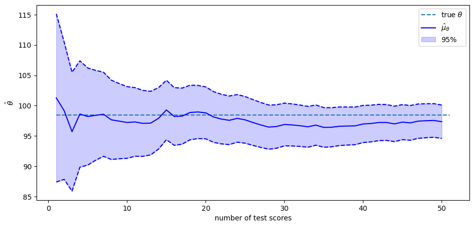
_images/bbdb443f534f5157e7c809f66a0fe26751565f308d62e0e3bfa2f3e46f8e37f0.png

The solid blue line in the plot above shows ${\hat{μ}}_{θ}$ as a function of the number of test scores that we have recorded and conditioned on.

The blue area shows the span that comes from adding or subtracting $1.96 {\hat{σ}}_{θ}$ from ${\hat{μ}}_{θ}$ .

Therefore, $95 %$ of the probability mass of the conditional distribution falls in this range.

The value of the random $θ$ that we drew is shown by the black dotted line.

As more and more test scores come in, our estimate of the person’s $θ$ become more and more reliable.

By staring at the changes in the conditional distributions, we see that adding more test scores makes $\hat{θ}$ settle down and approach $θ$ .

Thus, each $y_{i}$ adds information about $θ$ .

If we were to drive the number of tests $n \to + \infty$ , the conditional standard deviation ${\hat{σ}}_{θ}$ would converge to $0$ at rate $\frac{1}{n^{.5}}$ .

12.6. Information as Surprise #

By using a different representation, let’s look at things from a different perspective.

We can represent the random vector $X$ defined above as

X = μ_{θ} 1_{n + 1} + C ϵ, ϵ \sim N (0, I)

where $C$ is a lower triangular Cholesky factor of $Σ$ so that

Σ \equiv D D^{'} = C C^{'}

and

E ϵ ϵ^{'} = I .

It follows that

ϵ \sim N (0, I) .

Let $G = C^{- 1}$

$G$ is also lower triangular.

We can compute $ϵ$ from the formula

ϵ = G (X - μ_{θ} 1_{n + 1})

This formula confirms that the orthonormal vector $ϵ$ contains the same information as the non-orthogonal vector $(X - μ_{θ} 1_{n + 1})$ .

We can say that $ϵ$ is an orthogonal basis for $(X - μ_{θ} 1_{n + 1})$ .

Let $c_{i}$ be the $i$ th element in the last row of $C$ .

Then we can write

(12.1)#

θ = μ_{θ} + c_{1} ϵ_{1} + c_{2} ϵ_{2} + \dots + c_{n} ϵ_{n} + c_{n + 1} ϵ_{n + 1}

The mutual orthogonality of the $ϵ_{i}$ ’s provides us with an informative way to interpret them in light of equation (12.1).

Thus, relative to what is known from tests $i = 1, \dots, n - 1$ , $c_{i} ϵ_{i}$ is the amount of new information about $θ$ brought by the test number $i$ .

Here new information means surprise or what could not be predicted from earlier information.

Formula (12.1) also provides us with an enlightening way to express conditional means and conditional variances that we computed earlier.

In particular,

E [θ ∣ y_{1}, \dots, y_{k}] = μ_{θ} + c_{1} ϵ_{1} + \dots + c_{k} ϵ_{k}

and

V a r (θ ∣ y_{1}, \dots, y_{k}) = c_{k + 1}^{2} + c_{k + 2}^{2} + \dots + c_{n + 1}^{2} .

C = np.linalg.cholesky(Σ_IQ)
G = np.linalg.inv(C)

ε = G @ (x - μθ)

cε = C[n, :] * ε

# compute the sequence of μθ and Σθ conditional on y1, y2, ..., yk
μθ_hat_arr_C = np.array([np.sum(cε[:k+1]) for k in range(n)]) + μθ
Σθ_hat_arr_C = np.array([np.sum(C[n, i+1:n+1] ** 2) for i in range(n)])

To confirm that these formulas give the same answers that we computed earlier, we can compare the means and variances of $θ$ conditional on ${y_{i}}_{i = 1}^{k}$ with what we obtained above using the formulas implemented in the class MultivariateNormal built on our original representation of conditional distributions for multivariate normal distributions.

# conditional mean
np.max(np.abs(μθ_hat_arr - μθ_hat_arr_C)) < 1e-10

True

# conditional variance
np.max(np.abs(Σθ_hat_arr - Σθ_hat_arr_C)) < 1e-10

True

12.7. Cholesky Factor Magic #

Evidently, the Cholesky factorizations automatically computes the population regression coefficients and associated statistics that are produced by our MultivariateNormal class.

The Cholesky factorization computes these things recursively.

Indeed, in formula (12.1),

the random variable $c_{i} ϵ_{i}$ is information about $θ$ that is not contained by the information in $ϵ_{1}, ϵ_{2}, \dots, ϵ_{i - 1}$
the coefficient $c_{i}$ is the simple population regression coefficient of $θ - μ_{θ}$ on $ϵ_{i}$

12.8. Math and Verbal Intelligence #

We can alter the preceding example to be more realistic.

There is ample evidence that IQ is not a scalar.

Some people are good in math skills but poor in language skills.

Other people are good in language skills but poor in math skills.

So now we shall assume that there are two dimensions of IQ, $θ$ and $η$ .

These determine average performances in math and language tests, respectively.

We observe math scores ${y_{i}}_{i = 1}^{n}$ and language scores ${y_{i}}_{i = n + 1}^{2 n}$ .

When $n = 2$ , we assume that outcomes are draws from a multivariate normal distribution with representation

\begin{array}{r} X = [\begin{array}{c} y_{1} \\ y_{2} \\ y_{3} \\ y_{4} \\ θ \\ η \end{array}] = [\begin{array}{c} μ_{θ} \\ μ_{θ} \\ μ_{η} \\ μ_{η} \\ μ_{θ} \\ μ_{η} \end{array}] + [\begin{array}{cccccc} σ_{y} & 0 & 0 & 0 & σ_{θ} & 0 \\ 0 & σ_{y} & 0 & 0 & σ_{θ} & 0 \\ 0 & 0 & σ_{y} & 0 & 0 & σ_{η} \\ 0 & 0 & 0 & σ_{y} & 0 & σ_{η} \\ 0 & 0 & 0 & 0 & σ_{θ} & 0 \\ 0 & 0 & 0 & 0 & 0 & σ_{η} \end{array}] [\begin{array}{c} w_{1} \\ w_{2} \\ w_{3} \\ w_{4} \\ w_{5} \\ w_{6} \end{array}] \end{array}

where $w [\begin{matrix} w_{1} \\ w_{2} \\ ⋮ \\ w_{6} \end{matrix}]$ is a standard normal random vector.

We construct a Python function construct_moments_IQ2d to construct the mean vector and covariance matrix of the joint normal distribution.

def construct_moments_IQ2d(n, μθ, σθ, μη, ση, σy):

    μ_IQ2d = np.empty(2*(n+1))
    μ_IQ2d[:n] = μθ
    μ_IQ2d[2*n] = μθ
    μ_IQ2d[n:2*n] = μη
    μ_IQ2d[2*n+1] = μη


    D_IQ2d = np.zeros((2*(n+1), 2*(n+1)))
    D_IQ2d[range(2*n), range(2*n)] = σy
    D_IQ2d[:n, 2*n] = σθ
    D_IQ2d[2*n, 2*n] = σθ
    D_IQ2d[n:2*n, 2*n+1] = ση
    D_IQ2d[2*n+1, 2*n+1] = ση

    Σ_IQ2d = D_IQ2d @ D_IQ2d.T

    return μ_IQ2d, Σ_IQ2d, D_IQ2d

Let’s put the function to work.

n = 2
# mean and variance of θ, η, and y
μθ, σθ, μη, ση, σy = 100., 10., 100., 10, 10

μ_IQ2d, Σ_IQ2d, D_IQ2d = construct_moments_IQ2d(n, μθ, σθ, μη, ση, σy)
μ_IQ2d, Σ_IQ2d, D_IQ2d

(array([100., 100., 100., 100., 100., 100.]),
 array([[200., 100.,   0.,   0., 100.,   0.],
        [100., 200.,   0.,   0., 100.,   0.],
        [  0.,   0., 200., 100.,   0., 100.],
        [  0.,   0., 100., 200.,   0., 100.],
        [100., 100.,   0.,   0., 100.,   0.],
        [  0.,   0., 100., 100.,   0., 100.]]),
 array([[10.,  0.,  0.,  0., 10.,  0.],
        [ 0., 10.,  0.,  0., 10.,  0.],
        [ 0.,  0., 10.,  0.,  0., 10.],
        [ 0.,  0.,  0., 10.,  0., 10.],
        [ 0.,  0.,  0.,  0., 10.,  0.],
        [ 0.,  0.,  0.,  0.,  0., 10.]]))

# take one draw
x = np.random.multivariate_normal(μ_IQ2d, Σ_IQ2d)
y1 = x[:n]
y2 = x[n:2*n]
θ = x[2*n]
η = x[2*n+1]

# the true values
θ, η

(98.25677374913887, 101.41570209166122)

We first compute the joint normal distribution of $(θ, η)$ .

multi_normal_IQ2d = MultivariateNormal(μ_IQ2d, Σ_IQ2d)

k = 2*n # the length of data vector
multi_normal_IQ2d.partition(k)

multi_normal_IQ2d.cond_dist(1, [*y1, *y2])

(array([96.11974166, 97.0216911 ]),
 array([[33.33333333,  0.        ],
        [ 0.        , 33.33333333]]))

Now let’s compute distributions of $θ$ and $μ$ separately conditional on various subsets of test scores.

It will be fun to compare outcomes with the help of an auxiliary function cond_dist_IQ2d that we now construct.

def cond_dist_IQ2d(μ, Σ, data):

    n = len(μ)

    multi_normal = MultivariateNormal(μ, Σ)
    multi_normal.partition(n-1)
    μ_hat, Σ_hat = multi_normal.cond_dist(1, data)

    return μ_hat, Σ_hat

Let’s see how things work for an example.

for indices, IQ, conditions in [([*range(2*n), 2*n], 'θ', 'y1, y2, y3, y4'),
                                ([*range(n), 2*n], 'θ', 'y1, y2'),
                                ([*range(n, 2*n), 2*n], 'θ', 'y3, y4'),
                                ([*range(2*n), 2*n+1], 'η', 'y1, y2, y3, y4'),
                                ([*range(n), 2*n+1], 'η', 'y1, y2'),
                                ([*range(n, 2*n), 2*n+1], 'η', 'y3, y4')]:

    μ_hat, Σ_hat = cond_dist_IQ2d(μ_IQ2d[indices], Σ_IQ2d[indices][:, indices], x[indices[:-1]])
    print(f'The mean and variance of {IQ} conditional on {conditions: <15} are ' +
          f'{μ_hat[0]:1.2f} and {Σ_hat[0, 0]:1.2f} respectively')

The mean and variance of θ conditional on y1, y2, y3, y4  are 96.12 and 33.33 respectively
The mean and variance of θ conditional on y1, y2          are 96.12 and 33.33 respectively
The mean and variance of θ conditional on y3, y4          are 100.00 and 100.00 respectively
The mean and variance of η conditional on y1, y2, y3, y4  are 97.02 and 33.33 respectively
The mean and variance of η conditional on y1, y2          are 100.00 and 100.00 respectively
The mean and variance of η conditional on y3, y4          are 97.02 and 33.33 respectively

Evidently, math tests provide no information about $μ$ and language tests provide no information about $η$ .

12.9. Univariate Time Series Analysis #

We can use the multivariate normal distribution and a little matrix algebra to present foundations of univariate linear time series analysis.

Let $x_{t}, y_{t}, v_{t}, w_{t + 1}$ each be scalars for $t \geq 0$ .

Consider the following model:

\begin{array}{r} \begin{aligned} x_{0} & \sim N (0, σ_{0}^{2}) \\ x_{t + 1} & = a x_{t} + b w_{t + 1}, w_{t + 1} \sim N (0, 1), t \geq 0 \\ y_{t} & = c x_{t} + d v_{t}, v_{t} \sim N (0, 1), t \geq 0 \end{aligned} \end{array}

We can compute the moments of $x_{t}$

$E x_{t + 1}^{2} = a^{2} E x_{t}^{2} + b^{2}, t \geq 0$ , where $E x_{0}^{2} = σ_{0}^{2}$
$E x_{t + j} x_{t} = a^{j} E x_{t}^{2}, \forall t \forall j$

Given some $T$ , we can formulate the sequence ${x_{t}}_{t = 0}^{T}$ as a random vector

\begin{array}{r} X = [\begin{array}{c} x_{0} \\ x_{1} \\ ⋮ \\ x_{T} \end{array}] \end{array}

and the covariance matrix $Σ_{x}$ can be constructed using the moments we have computed above.

Similarly, we can define

\begin{array}{r} Y = [\begin{array}{c} y_{0} \\ y_{1} \\ ⋮ \\ y_{T} \end{array}], v = [\begin{array}{c} v_{0} \\ v_{1} \\ ⋮ \\ v_{T} \end{array}] \end{array}

and therefore

Y = C X + D V

where $C$ and $D$ are both diagonal matrices with constant $c$ and $d$ as diagonal respectively.

Consequently, the covariance matrix of $Y$ is

Σ_{y} = E Y Y^{'} = C Σ_{x} C^{'} + D D^{'}

By stacking $X$ and $Y$ , we can write

\begin{array}{r} Z = [\begin{array}{c} X \\ Y \end{array}] \end{array}

and

\begin{array}{r} Σ_{z} = E Z Z^{'} = [\begin{array}{cc} Σ_{x} & Σ_{x} C^{'} \\ C Σ_{x} & Σ_{y} \end{array}] \end{array}

Thus, the stacked sequences ${x_{t}}_{t = 0}^{T}$ and ${y_{t}}_{t = 0}^{T}$ jointly follow the multivariate normal distribution $N (0, Σ_{z})$ .

# as an example, consider the case where T = 3
T = 3

# variance of the initial distribution x_0
σ0 = 1.

# parameters of the equation system
a = .9
b = 1.
c = 1.0
d = .05

# construct the covariance matrix of X
Σx = np.empty((T+1, T+1))

Σx[0, 0] = σ0 ** 2
for i in range(T):
    Σx[i, i+1:] = Σx[i, i] * a ** np.arange(1, T+1-i)
    Σx[i+1:, i] = Σx[i, i+1:]

    Σx[i+1, i+1] = a ** 2 * Σx[i, i] + b ** 2

Σx

array([[1.      , 0.9     , 0.81    , 0.729   ],
       [0.9     , 1.81    , 1.629   , 1.4661  ],
       [0.81    , 1.629   , 2.4661  , 2.21949 ],
       [0.729   , 1.4661  , 2.21949 , 2.997541]])

# construct the covariance matrix of Y
C = np.eye(T+1) * c
D = np.eye(T+1) * d

Σy = C @ Σx @ C.T + D @ D.T

# construct the covariance matrix of Z
Σz = np.empty((2*(T+1), 2*(T+1)))

Σz[:T+1, :T+1] = Σx
Σz[:T+1, T+1:] = Σx @ C.T
Σz[T+1:, :T+1] = C @ Σx
Σz[T+1:, T+1:] = Σy

Σz

array([[1.      , 0.9     , 0.81    , 0.729   , 1.      , 0.9     ,
        0.81    , 0.729   ],
       [0.9     , 1.81    , 1.629   , 1.4661  , 0.9     , 1.81    ,
        1.629   , 1.4661  ],
       [0.81    , 1.629   , 2.4661  , 2.21949 , 0.81    , 1.629   ,
        2.4661  , 2.21949 ],
       [0.729   , 1.4661  , 2.21949 , 2.997541, 0.729   , 1.4661  ,
        2.21949 , 2.997541],
       [1.      , 0.9     , 0.81    , 0.729   , 1.0025  , 0.9     ,
        0.81    , 0.729   ],
       [0.9     , 1.81    , 1.629   , 1.4661  , 0.9     , 1.8125  ,
        1.629   , 1.4661  ],
       [0.81    , 1.629   , 2.4661  , 2.21949 , 0.81    , 1.629   ,
        2.4686  , 2.21949 ],
       [0.729   , 1.4661  , 2.21949 , 2.997541, 0.729   , 1.4661  ,
        2.21949 , 3.000041]])

# construct the mean vector of Z
μz = np.zeros(2*(T+1))

The following Python code lets us sample random vectors $X$ and $Y$ .

This is going to be very useful for doing the conditioning to be used in the fun exercises below.

z = np.random.multivariate_normal(μz, Σz)

x = z[:T+1]
y = z[T+1:]

12.9.1. Smoothing Example#

This is an instance of a classic smoothing calculation whose purpose is to compute $E X ∣ Y$ .

An interpretation of this example is

$X$ is a random sequence of hidden Markov state variables $x_{t}$
$Y$ is a sequence of observed signals $y_{t}$ bearing information about the hidden state

# construct a MultivariateNormal instance
multi_normal_ex1 = MultivariateNormal(μz, Σz)
x = z[:T+1]
y = z[T+1:]

# partition Z into X and Y
multi_normal_ex1.partition(T+1)

# compute the conditional mean and covariance matrix of X given Y=y

print("X = ", x)
print("Y = ", y)
print(" E [ X | Y] = ", )

multi_normal_ex1.cond_dist(0, y)

X =  [-1.72795143 -0.7321461  -3.84659701 -4.2759139 ]
Y =  [-1.77368314 -0.72845598 -3.84781329 -4.30029643]
 E [ X | Y] =

(array([-1.76734581, -0.7377382 , -3.84176018, -4.2981949 ]),
 array([[2.48875094e-03, 5.57449314e-06, 1.24861729e-08, 2.80235835e-11],
        [5.57449314e-06, 2.48876343e-03, 5.57452116e-06, 1.25113941e-08],
        [1.24861729e-08, 5.57452116e-06, 2.48876346e-03, 5.58575339e-06],
        [2.80235835e-11, 1.25113941e-08, 5.58575339e-06, 2.49377812e-03]]))

12.9.2. Filtering Exercise#

Compute $E [x_{t} ∣ y_{t - 1}, y_{t - 2}, \dots, y_{0}]$ .

To do so, we need to first construct the mean vector and the covariance matrix of the subvector $[x_{t}, y_{0}, \dots, y_{t - 2}, y_{t - 1}]$ .

For example, let’s say that we want the conditional distribution of $x_{3}$ .

t = 3

# mean of the subvector
sub_μz = np.zeros(t+1)

# covariance matrix of the subvector
sub_Σz = np.empty((t+1, t+1))

sub_Σz[0, 0] = Σz[t, t] # x_t
sub_Σz[0, 1:] = Σz[t, T+1:T+t+1]
sub_Σz[1:, 0] = Σz[T+1:T+t+1, t]
sub_Σz[1:, 1:] = Σz[T+1:T+t+1, T+1:T+t+1]

sub_Σz

array([[2.997541, 0.729   , 1.4661  , 2.21949 ],
       [0.729   , 1.0025  , 0.9     , 0.81    ],
       [1.4661  , 0.9     , 1.8125  , 1.629   ],
       [2.21949 , 0.81    , 1.629   , 2.4686  ]])

multi_normal_ex2 = MultivariateNormal(sub_μz, sub_Σz)
multi_normal_ex2.partition(1)

sub_y = y[:t]

multi_normal_ex2.cond_dist(0, sub_y)

(array([-3.45588616]), array([[1.00201996]]))

12.9.3. Prediction Exercise#

Compute $E [y_{t} ∣ y_{t - j}, \dots, y_{0}]$ .

As what we did in exercise 2, we will construct the mean vector and covariance matrix of the subvector $[y_{t}, y_{0}, \dots, y_{t - j - 1}, y_{t - j}]$ .

For example, we take a case in which $t = 3$ and $j = 2$ .

t = 3
j = 2

sub_μz = np.zeros(t-j+2)
sub_Σz = np.empty((t-j+2, t-j+2))

sub_Σz[0, 0] = Σz[T+t+1, T+t+1]
sub_Σz[0, 1:] = Σz[T+t+1, T+1:T+t-j+2]
sub_Σz[1:, 0] = Σz[T+1:T+t-j+2, T+t+1]
sub_Σz[1:, 1:] = Σz[T+1:T+t-j+2, T+1:T+t-j+2]

sub_Σz

array([[3.000041, 0.729   , 1.4661  ],
       [0.729   , 1.0025  , 0.9     ],
       [1.4661  , 0.9     , 1.8125  ]])

multi_normal_ex3 = MultivariateNormal(sub_μz, sub_Σz)
multi_normal_ex3.partition(1)

sub_y = y[:t-j+1]

multi_normal_ex3.cond_dist(0, sub_y)

(array([-0.59179082]), array([[1.81413617]]))

12.9.4. Constructing a Wold Representation#

Now we’ll apply Cholesky decomposition to decompose $Σ_{y} = H H^{'}$ and form

ϵ = H^{- 1} Y .

Then we can represent $y_{t}$ as

y_{t} = h_{t, t} ϵ_{t} + h_{t, t - 1} ϵ_{t - 1} + \dots + h_{t, 0} ϵ_{0} .

H = np.linalg.cholesky(Σy)

H

array([[1.00124922, 0.        , 0.        , 0.        ],
       [0.8988771 , 1.00225743, 0.        , 0.        ],
       [0.80898939, 0.89978675, 1.00225743, 0.        ],
       [0.72809046, 0.80980808, 0.89978676, 1.00225743]])

ε = np.linalg.inv(H) @ y

ε

array([-1.77147019,  0.86193226, -3.18308234, -0.84250836])

array([-1.77368314, -0.72845598, -3.84781329, -4.30029643])

This example is an instance of what is known as a Wold representation in time series analysis.

12.10. Stochastic Difference Equation #

Consider the stochastic second-order linear difference equation

y_{t} = α_{0} + α_{1} y_{y - 1} + α_{2} y_{t - 2} + u_{t}

where $u_{t} \sim N (0, σ_{u}^{2})$ and

\begin{array}{r} [\begin{array}{c} y_{- 1} \\ y_{0} \end{array}] \sim N (μ_{\tilde{y}}, Σ_{\tilde{y}}) \end{array}

It can be written as a stacked system

\begin{array}{r} \underset{\equiv A}{\underset{⏟}{[\begin{array}{cccccccc} 1 & 0 & 0 & 0 & \dots & 0 & 0 & 0 \\ - α_{1} & 1 & 0 & 0 & \dots & 0 & 0 & 0 \\ - α_{2} & - α_{1} & 1 & 0 & \dots & 0 & 0 & 0 \\ 0 & - α_{2} & - α_{1} & 1 & \dots & 0 & 0 & 0 \\ ⋮ & ⋮ & ⋮ & ⋮ & \dots & ⋮ & ⋮ & ⋮ \\ 0 & 0 & 0 & 0 & \dots & - α_{2} & - α_{1} & 1 \end{array}]}} [\begin{array}{c} y_{1} \\ y_{2} \\ y_{3} \\ y_{4} \\ ⋮ \\ y_{T} \end{array}] = \underset{\equiv b}{\underset{⏟}{[\begin{array}{c} α_{0} + α_{1} y_{0} + α_{2} y_{- 1} \\ α_{0} + α_{2} y_{0} \\ α_{0} \\ α_{0} \\ ⋮ \\ α_{0} \end{array}]}} + \underset{\equiv u}{\underset{⏟}{[\begin{array}{c} u_{1} \\ u_{2} \\ u_{3} \\ u_{4} \\ ⋮ \\ u_{T} \end{array}]}} \end{array}

We can compute $y$ by solving the system

y = A^{- 1} (b + u)

We have

\begin{array}{r} \begin{aligned} μ_{y} = A^{- 1} μ_{b} \\ Σ_{y} & = A^{- 1} E [(b - μ_{b} + u) {(b - μ_{b} + u)}^{'}] {(A^{- 1})}^{'} \\ = A^{- 1} (Σ_{b} + Σ_{u}) {(A^{- 1})}^{'} \end{aligned} \end{array}

where

\begin{array}{r} μ_{b} = [\begin{array}{c} α_{0} + α_{1} μ_{y_{0}} + α_{2} μ_{y_{- 1}} \\ α_{0} + α_{2} μ_{y_{0}} \\ α_{0} \\ ⋮ \\ α_{0} \end{array}] \end{array}

\begin{array}{r} Σ_{b} = [\begin{array}{cc} C Σ_{\tilde{y}} C^{'} & 0_{N - 2 \times N - 2} \\ 0_{N - 2 \times 2} & 0_{N - 2 \times N - 2} \end{array}], C = [\begin{array}{cc} α_{2} & α_{1} \\ 0 & α_{2} \end{array}] \end{array}

\begin{array}{r} Σ_{u} = [\begin{array}{cccc} σ_{u}^{2} & 0 & \dots & 0 \\ 0 & σ_{u}^{2} & \dots & 0 \\ ⋮ & ⋮ & ⋮ & ⋮ \\ 0 & 0 & \dots & σ_{u}^{2} \end{array}] \end{array}

# set parameters
T = 80
T = 160
# coefficients of the second order difference equation
𝛼0 = 10
𝛼1 = 1.53
𝛼2 = -.9

# variance of u
σu = 1.
σu = 10.

# distribution of y_{-1} and y_{0}
μy_tilde = np.array([1., 0.5])
Σy_tilde = np.array([[2., 1.], [1., 0.5]])

# construct A and A^{\prime}
A = np.zeros((T, T))

for i in range(T):
    A[i, i] = 1

    if i-1 >= 0:
        A[i, i-1] = -𝛼1

    if i-2 >= 0:
        A[i, i-2] = -𝛼2

A_inv = np.linalg.inv(A)

# compute the mean vectors of b and y
μb = np.full(T, 𝛼0)
μb[0] += 𝛼1 * μy_tilde[1] + 𝛼2 * μy_tilde[0]
μb[1] += 𝛼2 * μy_tilde[1]

μy = A_inv @ μb

# compute the covariance matrices of b and y
Σu = np.eye(T) * σu ** 2

Σb = np.zeros((T, T))

C = np.array([[𝛼2, 𝛼1], [0, 𝛼2]])
Σb[:2, :2] = C @ Σy_tilde @ C.T

Σy = A_inv @ (Σb + Σu) @ A_inv.T

12.11. Application to Stock Price Model #

Let

p_{t} = \sum_{j = 0}^{T - t} β^{j} y_{t + j}

Form

\begin{array}{r} \underset{\equiv p}{\underset{⏟}{[\begin{array}{c} p_{1} \\ p_{2} \\ p_{3} \\ ⋮ \\ p_{T} \end{array}]}} = \underset{\equiv B}{\underset{⏟}{[\begin{array}{ccccc} 1 & β & β^{2} & \dots & β^{T - 1} \\ 0 & 1 & β & \dots & β^{T - 2} \\ 0 & 0 & 1 & \dots & β^{T - 3} \\ ⋮ & ⋮ & ⋮ & ⋮ & ⋮ \\ 0 & 0 & 0 & \dots & 1 \end{array}]}} [\begin{array}{c} y_{1} \\ y_{2} \\ y_{3} \\ ⋮ \\ y_{T} \end{array}] \end{array}

we have

\begin{array}{r} \begin{matrix} μ_{p} = B μ_{y} \\ Σ_{p} = B Σ_{y} B^{'} \end{matrix} \end{array}

β = .96

# construct B
B = np.zeros((T, T))

for i in range(T):
    B[i, i:] = β ** np.arange(0, T-i)

Denote

\begin{array}{r} z = [\begin{array}{c} y \\ p \end{array}] = \underset{\equiv D}{\underset{⏟}{[\begin{array}{c} I \\ B \end{array}]}} y \end{array}

Thus, ${y_{t}}_{t = 1}^{T}$ and ${p_{t}}_{t = 1}^{T}$ jointly follow the multivariate normal distribution $N (μ_{z}, Σ_{z})$ , where

μ_{z} = D μ_{y}

Σ_{z} = D Σ_{y} D^{'}

D = np.vstack([np.eye(T), B])

μz = D @ μy
Σz = D @ Σy @ D.T

We can simulate paths of $y_{t}$ and $p_{t}$ and compute the conditional mean $E [p_{t} ∣ y_{t - 1}, y_{t}]$ using the MultivariateNormal class.

z = np.random.multivariate_normal(μz, Σz)
y, p = z[:T], z[T:]

cond_Ep = np.empty(T-1)

sub_μ = np.empty(3)
sub_Σ = np.empty((3, 3))
for t in range(2, T+1):
    sub_μ[:] = μz[[t-2, t-1, T-1+t]]
    sub_Σ[:, :] = Σz[[t-2, t-1, T-1+t], :][:, [t-2, t-1, T-1+t]]

    multi_normal = MultivariateNormal(sub_μ, sub_Σ)
    multi_normal.partition(2)

    cond_Ep[t-2] = multi_normal.cond_dist(1, y[t-2:t])[0][0]

plt.plot(range(1, T), y[1:], label='$y_{t}$')
plt.plot(range(1, T), y[:-1], label='$y_{t-1}$')
plt.plot(range(1, T), p[1:], label='$p_{t}$')
plt.plot(range(1, T), cond_Ep, label='$Ep_{t}|y_{t}, y_{t-1}$')

plt.xlabel('t')
plt.legend(loc=1)
plt.show()

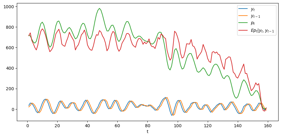
_images/460c6345256d13d0985dc23c47fa3850ce93e1e86ec86fb037acd5f07dea4295.png

In the above graph, the green line is what the price of the stock would be if people had perfect foresight about the path of dividends while the green line is the conditional expectation $E p_{t} | y_{t}, y_{t - 1}$ , which is what the price would be if people did not have perfect foresight but were optimally predicting future dividends on the basis of the information $y_{t}, y_{t - 1}$ at time $t$ .

12.12. Filtering Foundations #

Assume that $x_{0}$ is an $n \times 1$ random vector and that $y_{0}$ is a $p \times 1$ random vector determined by the observation equation

y_{0} = G x_{0} + v_{0}, x_{0} \sim N ({\hat{x}}_{0}, Σ_{0}), v_{0} \sim N (0, R)

where $v_{0}$ is orthogonal to $x_{0}$ , $G$ is a $p \times n$ matrix, and $R$ is a $p \times p$ positive definite matrix.

We consider the problem of someone who

observes $y_{0}$
does not observe $x_{0}$ ,
knows ${\hat{x}}_{0}, Σ_{0}, G, R$ and therefore the joint probability distribution of the vector $[\begin{matrix} x_{0} \\ y_{0} \end{matrix}]$
wants to infer $x_{0}$ from $y_{0}$ in light of what he knows about that joint probability distribution.

Therefore, the person wants to construct the probability distribution of $x_{0}$ conditional on the random vector $y_{0}$ .

The joint distribution of $[\begin{matrix} x_{0} \\ y_{0} \end{matrix}]$ is multivariate normal $N (μ, Σ)$ with

μ = [\begin{matrix} {\hat{x}}_{0} \\ G {\hat{x}}_{0} \end{matrix}], Σ = [\begin{matrix} Σ_{0} & Σ_{0} G^{'} \\ G Σ_{0} & G Σ_{0} G^{'} + R \end{matrix}]

By applying an appropriate instance of the above formulas for the mean vector ${\hat{μ}}_{1}$ and covariance matrix ${\hat{Σ}}_{11}$ of $z_{1}$ conditional on $z_{2}$ , we find that the probability distribution of $x_{0}$ conditional on $y_{0}$ is $N ({\tilde{x}}_{0}, {\tilde{Σ}}_{0})$ where

\begin{aligned} β_{0} & = Σ_{0} G^{'} (G Σ_{0} G^{'} + R)^{- 1} \\ {\tilde{x}}_{0} & = {\hat{x}}_{0} + β_{0} (y_{0} - G {\hat{x}}_{0}) \\ {\tilde{Σ}}_{0} & = Σ_{0} - Σ_{0} G^{'} (G Σ_{0} G^{'} + R)^{- 1} G Σ_{0} \end{aligned}

We can express our finding that the probability distribution of $x_{0}$ conditional on $y_{0}$ is $N ({\tilde{x}}_{0}, {\tilde{Σ}}_{0})$ by representing $x_{0}$ as

(12.2)#

x_{0} = {\tilde{x}}_{0} + ζ_{0}

where $ζ_{0}$ is a Gaussian random vector that is orthogonal to ${\tilde{x}}_{0}$ and $y_{0}$ and that has mean vector $0$ and conditional covariance matrix $E [ζ_{0} ζ_{0}^{'} | y_{0}] = {\tilde{Σ}}_{0}$ .

12.12.1. Step toward dynamics#

Now suppose that we are in a time series setting and that we have the one-step state transition equation

x_{1} = A x_{0} + C w_{1}, w_{1} \sim N (0, I)

where $A$ is an $n \times n$ matrix and $C$ is an $n \times m$ matrix.

Using equation (12.2), we can also represent $x_{1}$ as

x_{1} = A ({\tilde{x}}_{0} + ζ_{0}) + C w_{1}

It follows that

E x_{1} | y_{0} = A {\tilde{x}}_{0}

and that the corresponding conditional covariance matrix $E (x_{1} - E x_{1} | y_{0}) (x_{1} - E x_{1} | y_{0})^{'} \equiv Σ_{1}$ is

Σ_{1} = A {\tilde{Σ}}_{0} A^{'} + C C^{'}

Σ_{1} = A Σ_{0} A^{'} - A Σ_{0} G^{'} (G Σ_{0} G^{'} + R)^{- 1} G Σ_{0} A^{'}

We can write the mean of $x_{1}$ conditional on $y_{0}$ as

{\hat{x}}_{1} = A {\hat{x}}_{0} + A Σ_{0} G^{'} (G Σ_{0} G^{'} + R)^{- 1} (y_{0} - G {\hat{x}}_{0})

{\hat{x}}_{1} = A {\hat{x}}_{0} + K_{0} (y_{0} - G {\hat{x}}_{0})

where

K_{0} = A Σ_{0} G^{'} (G Σ_{0} G^{'} + R)^{- 1}

12.12.2. Dynamic version#

Suppose now that for $t \geq 0$ , ${x_{t + 1}, y_{t}}_{t = 0}^{\infty}$ are governed by the equations

\begin{aligned} x_{t + 1} & = A x_{t} + C w_{t + 1} \\ y_{t} & = G x_{t} + v_{t} \end{aligned}

where as before $x_{0} \sim N ({\hat{x}}_{0}, Σ_{0})$ , $w_{t + 1}$ is the $t + 1$ th component of an i.i.d. stochastic process distributed as $w_{t + 1} \sim N (0, I)$ , and $v_{t}$ is the $t$ th component of an i.i.d. process distributed as $v_{t} \sim N (0, R)$ and the ${w_{t + 1}}_{t = 0}^{\infty}$ and ${v_{t}}_{t = 0}^{\infty}$ processes are orthogonal at all pairs of dates.

The logic and formulas that we applied above imply that the probability distribution of $x_{t}$ conditional on $y_{0}, y_{1}, \dots, y_{t - 1} = y^{t - 1}$ is

x_{t} | y^{t - 1} \sim N (A {\tilde{x}}_{t}, A {\tilde{Σ}}_{t} A^{'} + C C^{'})

where ${{\tilde{x}}_{t}, {\tilde{Σ}}_{t}}_{t = 1}^{\infty}$ can be computed by iterating on the following equations starting from $t = 1$ and initial conditions for ${\tilde{x}}_{0}, {\tilde{Σ}}_{0}$ computed as we have above:

\begin{aligned} Σ_{t} & = A {\tilde{Σ}}_{t - 1} A^{'} + C C^{'} \\ {\hat{x}}_{t} & = A {\tilde{x}}_{t - 1} \\ β_{t} & = Σ_{t} G^{'} (G Σ_{t} G^{'} + R)^{- 1} \\ {\tilde{x}}_{t} & = {\hat{x}}_{t} + β_{t} (y_{t} - G {\hat{x}}_{t}) \\ {\tilde{Σ}}_{t} & = Σ_{t} - Σ_{t} G^{'} (G Σ_{t} G^{'} + R)^{- 1} G Σ_{t} \end{aligned}

If we shift the first equation forward one period and then substitute the expression for ${\tilde{Σ}}_{t}$ on the right side of the fifth equation into it we obtain

Σ_{t + 1} = C C^{'} + A Σ_{t} A^{'} - A Σ_{t} G^{'} (G Σ_{t} G^{'} + R)^{- 1} G Σ_{t} A^{'} .

This is a matrix Riccati difference equation that is closely related to another matrix Riccati difference equation that appears in a quantecon lecture on the basics of linear quadratic control theory.

That equation has the form

P_{t - 1} = R + A^{'} P_{t} A - A^{'} P_{t} B (B^{'} P_{t} B + Q)^{- 1} B^{'} P_{t} A .

Stare at the two preceding equations for a moment or two, the first being a matrix difference equation for a conditional covariance matrix, the second being a matrix difference equation in the matrix appearing in a quadratic form for an intertemporal cost of value function.

Although the two equations are not identical, they display striking family resemblences.

the first equation tells dynamics that work forward in time
the second equation tells dynamics that work backward in time
while many of the terms are similar, one equation seems to apply matrix transformations to some matrices that play similar roles in the other equation

The family resemblences of these two equations reflects a transcendent duality that prevails between control theory and filtering theory.

12.12.3. An example#

We can use the Python class MultivariateNormal to construct examples.

Here is an example for a single period problem at time $0$

G = np.array([[1., 3.]])
R = np.array([[1.]])

x0_hat = np.array([0., 1.])
Σ0 = np.array([[1., .5], [.3, 2.]])

μ = np.hstack([x0_hat, G @ x0_hat])
Σ = np.block([[Σ0, Σ0 @ G.T], [G @ Σ0, G @ Σ0 @ G.T + R]])

# construction of the multivariate normal instance
multi_normal = MultivariateNormal(μ, Σ)

multi_normal.partition(2)

# the observation of y
y0 = 2.3

# conditional distribution of x0
μ1_hat, Σ11 = multi_normal.cond_dist(0, y0)
μ1_hat, Σ11

(array([-0.078125,  0.803125]),
 array([[ 0.72098214, -0.203125  ],
        [-0.403125  ,  0.228125  ]]))

A = np.array([[0.5, 0.2], [-0.1, 0.3]])
C = np.array([[2.], [1.]])

# conditional distribution of x1
x1_cond = A @ μ1_hat
Σ1_cond = C @ C.T + A @ Σ11 @ A.T
x1_cond, Σ1_cond

(array([0.1215625, 0.24875  ]),
 array([[4.12874554, 1.95523214],
        [1.92123214, 1.04592857]]))

12.12.4. Code for Iterating#

Here is code for solving a dynamic filtering problem by iterating on our equations, followed by an example.

def iterate(x0_hat, Σ0, A, C, G, R, y_seq):

    p, n = G.shape

    T = len(y_seq)
    x_hat_seq = np.empty((T+1, n))
    Σ_hat_seq = np.empty((T+1, n, n))

    x_hat_seq[0] = x0_hat
    Σ_hat_seq[0] = Σ0

    for t in range(T):
        xt_hat = x_hat_seq[t]
        Σt = Σ_hat_seq[t]
        μ = np.hstack([xt_hat, G @ xt_hat])
        Σ = np.block([[Σt, Σt @ G.T], [G @ Σt, G @ Σt @ G.T + R]])

        # filtering
        multi_normal = MultivariateNormal(μ, Σ)
        multi_normal.partition(n)
        x_tilde, Σ_tilde = multi_normal.cond_dist(0, y_seq[t])

        # forecasting
        x_hat_seq[t+1] = A @ x_tilde
        Σ_hat_seq[t+1] = C @ C.T + A @ Σ_tilde @ A.T

    return x_hat_seq, Σ_hat_seq

iterate(x0_hat, Σ0, A, C, G, R, [2.3, 1.2, 3.2])

(array([[0.        , 1.        ],
        [0.1215625 , 0.24875   ],
        [0.18680212, 0.06904689],
        [0.75576875, 0.05558463]]),
 array([[[1.        , 0.5       ],
         [0.3       , 2.        ]],
 
        [[4.12874554, 1.95523214],
         [1.92123214, 1.04592857]],
 
        [[4.08198663, 1.99218488],
         [1.98640488, 1.00886423]],
 
        [[4.06457628, 2.00041999],
         [1.99943739, 1.00275526]]]))

The iterative algorithm just described is a version of the celebrated Kalman filter.

We describe the Kalman filter and some applications of it in A First Look at the Kalman Filter

12.13. Classic Factor Analysis Model #

The factor analysis model widely used in psychology and other fields can be represented as

Y = Λ f + U

where

$Y$ is $n \times 1$ random vector, $E U U^{'} = D$ is a diagonal matrix,
$Λ$ is $n \times k$ coefficient matrix,
$f$ is $k \times 1$ random vector, $E f f^{'} = I$ ,
$U$ is $n \times 1$ random vector, and $U ⊥ f$ (i.e., $E U f^{'} = 0$ )
It is presumed that $k$ is small relative to $n$ ; often $k$ is only $1$ or $2$ , as in our IQ examples.

This implies that

\begin{array}{r} \begin{matrix} Σ_{y} = E Y Y^{'} = Λ Λ^{'} + D \\ E Y f^{'} = Λ \\ E f Y^{'} = Λ^{'} \end{matrix} \end{array}

Thus, the covariance matrix $Σ_{Y}$ is the sum of a diagonal matrix $D$ and a positive semi-definite matrix $Λ Λ^{'}$ of rank $k$ .

This means that all covariances among the $n$ components of the $Y$ vector are intermediated by their common dependencies on the $k <$ factors.

Form

\begin{array}{r} Z = (\begin{array}{c} f \\ Y \end{array}) \end{array}

the covariance matrix of the expanded random vector $Z$ can be computed as

\begin{array}{r} Σ_{z} = E Z Z^{'} = (\begin{array}{cc} I & Λ^{'} \\ Λ & Λ Λ^{'} + D \end{array}) \end{array}

In the following, we first construct the mean vector and the covariance matrix for the case where $N = 10$ and $k = 2$ .

N = 10
k = 2

We set the coefficient matrix $Λ$ and the covariance matrix of $U$ to be

\begin{array}{r} Λ = (\begin{array}{cc} 1 & 0 \\ ⋮ & ⋮ \\ 1 & 0 \\ 0 & 1 \\ ⋮ & ⋮ \\ 0 & 1 \end{array}), D = (\begin{array}{cccc} σ_{u}^{2} & 0 & \dots & 0 \\ 0 & σ_{u}^{2} & \dots & 0 \\ ⋮ & ⋮ & ⋮ & ⋮ \\ 0 & 0 & \dots & σ_{u}^{2} \end{array}) \end{array}

where the first half of the first column of $Λ$ is filled with $1$ s and $0$ s for the rest half, and symmetrically for the second column.

$D$ is a diagonal matrix with parameter $σ_{u}^{2}$ on the diagonal.

Λ = np.zeros((N, k))
Λ[:N//2, 0] = 1
Λ[N//2:, 1] = 1

σu = .5
D = np.eye(N) * σu ** 2

# compute Σy
Σy = Λ @ Λ.T + D

We can now construct the mean vector and the covariance matrix for $Z$ .

μz = np.zeros(k+N)

Σz = np.empty((k+N, k+N))

Σz[:k, :k] = np.eye(k)
Σz[:k, k:] = Λ.T
Σz[k:, :k] = Λ
Σz[k:, k:] = Σy

z = np.random.multivariate_normal(μz, Σz)

f = z[:k]
y = z[k:]

multi_normal_factor = MultivariateNormal(μz, Σz)
multi_normal_factor.partition(k)

Let’s compute the conditional distribution of the hidden factor $f$ on the observations $Y$ , namely, $f ∣ Y = y$ .

multi_normal_factor.cond_dist(0, y)

(array([-1.14557316,  0.38088811]),
 array([[0.04761905, 0.        ],
        [0.        , 0.04761905]]))

We can verify that the conditional mean $E [f ∣ Y = y] = B Y$ where $B = Λ^{'} Σ_{y}^{- 1}$ .

B = Λ.T @ np.linalg.inv(Σy)

B @ y

array([-1.14557316,  0.38088811])

Similarly, we can compute the conditional distribution $Y ∣ f$ .

multi_normal_factor.cond_dist(1, f)

(array([-1.13919269, -1.13919269, -1.13919269, -1.13919269, -1.13919269,
         0.38187477,  0.38187477,  0.38187477,  0.38187477,  0.38187477]),
 array([[0.25, 0.  , 0.  , 0.  , 0.  , 0.  , 0.  , 0.  , 0.  , 0.  ],
        [0.  , 0.25, 0.  , 0.  , 0.  , 0.  , 0.  , 0.  , 0.  , 0.  ],
        [0.  , 0.  , 0.25, 0.  , 0.  , 0.  , 0.  , 0.  , 0.  , 0.  ],
        [0.  , 0.  , 0.  , 0.25, 0.  , 0.  , 0.  , 0.  , 0.  , 0.  ],
        [0.  , 0.  , 0.  , 0.  , 0.25, 0.  , 0.  , 0.  , 0.  , 0.  ],
        [0.  , 0.  , 0.  , 0.  , 0.  , 0.25, 0.  , 0.  , 0.  , 0.  ],
        [0.  , 0.  , 0.  , 0.  , 0.  , 0.  , 0.25, 0.  , 0.  , 0.  ],
        [0.  , 0.  , 0.  , 0.  , 0.  , 0.  , 0.  , 0.25, 0.  , 0.  ],
        [0.  , 0.  , 0.  , 0.  , 0.  , 0.  , 0.  , 0.  , 0.25, 0.  ],
        [0.  , 0.  , 0.  , 0.  , 0.  , 0.  , 0.  , 0.  , 0.  , 0.25]]))

It can be verified that the mean is $Λ I^{- 1} f = Λ f$ .

Λ @ f

array([-1.13919269, -1.13919269, -1.13919269, -1.13919269, -1.13919269,
        0.38187477,  0.38187477,  0.38187477,  0.38187477,  0.38187477])

12.14. PCA and Factor Analysis #

To learn about Principal Components Analysis (PCA), please see this lecture Singular Value Decompositions.

For fun, let’s apply a PCA decomposition to a covariance matrix $Σ_{y}$ that in fact is governed by our factor-analytic model.

Technically, this means that the PCA model is misspecified. (Can you explain why?)

Nevertheless, this exercise will let us study how well the first two principal components from a PCA can approximate the conditional expectations $E f_{i} | Y$ for our two factors $f_{i}$ , $i = 1, 2$ for the factor analytic model that we have assumed truly governs the data on $Y$ we have generated.

So we compute the PCA decomposition

Σ_{y} = P \tilde{Λ} P^{'}

where $\tilde{Λ}$ is a diagonal matrix.

We have

Y = P ϵ

and

ϵ = P^{'} Y

Note that we will arrange the eigenvectors in $P$ in the descending order of eigenvalues.

𝜆_tilde, P = np.linalg.eigh(Σy)

# arrange the eigenvectors by eigenvalues
ind = sorted(range(N), key=lambda x: 𝜆_tilde[x], reverse=True)

P = P[:, ind]
𝜆_tilde = 𝜆_tilde[ind]
Λ_tilde = np.diag(𝜆_tilde)

print('𝜆_tilde =', 𝜆_tilde)

𝜆_tilde = [5.25 5.25 0.25 0.25 0.25 0.25 0.25 0.25 0.25 0.25]

# verify the orthogonality of eigenvectors
np.abs(P @ P.T - np.eye(N)).max()

4.440892098500626e-16

# verify the eigenvalue decomposition is correct
P @ Λ_tilde @ P.T

array([[1.25, 1.  , 1.  , 1.  , 1.  , 0.  , 0.  , 0.  , 0.  , 0.  ],
       [1.  , 1.25, 1.  , 1.  , 1.  , 0.  , 0.  , 0.  , 0.  , 0.  ],
       [1.  , 1.  , 1.25, 1.  , 1.  , 0.  , 0.  , 0.  , 0.  , 0.  ],
       [1.  , 1.  , 1.  , 1.25, 1.  , 0.  , 0.  , 0.  , 0.  , 0.  ],
       [1.  , 1.  , 1.  , 1.  , 1.25, 0.  , 0.  , 0.  , 0.  , 0.  ],
       [0.  , 0.  , 0.  , 0.  , 0.  , 1.25, 1.  , 1.  , 1.  , 1.  ],
       [0.  , 0.  , 0.  , 0.  , 0.  , 1.  , 1.25, 1.  , 1.  , 1.  ],
       [0.  , 0.  , 0.  , 0.  , 0.  , 1.  , 1.  , 1.25, 1.  , 1.  ],
       [0.  , 0.  , 0.  , 0.  , 0.  , 1.  , 1.  , 1.  , 1.25, 1.  ],
       [0.  , 0.  , 0.  , 0.  , 0.  , 1.  , 1.  , 1.  , 1.  , 1.25]])

ε = P.T @ y

print("ε = ", ε)

ε =  [-2.68965844  0.89427629  0.79340353 -0.37962072 -0.82827448  0.65842092
 -0.03788382 -0.64394189  0.61617964  0.27127267]

# print the values of the two factors

print('f = ', f)

f =  [-1.13919269  0.38187477]

Below we’ll plot several things

the $N$ values of $y$
the $N$ values of the principal components $ϵ$
the value of the first factor $f_{1}$ plotted only for the first $N / 2$ observations of $y$ for which it receives a non-zero loading in $Λ$
the value of the second factor $f_{2}$ plotted only for the final $N / 2$ observations for which it receives a non-zero loading in $Λ$

plt.scatter(range(N), y, label='y')
plt.scatter(range(N), ε, label='$\epsilon$')
plt.hlines(f[0], 0, N//2-1, ls='--', label='$f_{1}$')
plt.hlines(f[1], N//2, N-1, ls='-.', label='$f_{2}$')
plt.legend()

plt.show()

<>:2: SyntaxWarning: invalid escape sequence '\e'
<>:2: SyntaxWarning: invalid escape sequence '\e'
/tmp/ipykernel_8076/2845509298.py:2: SyntaxWarning: invalid escape sequence '\e'
  plt.scatter(range(N), ε, label='$\epsilon$')

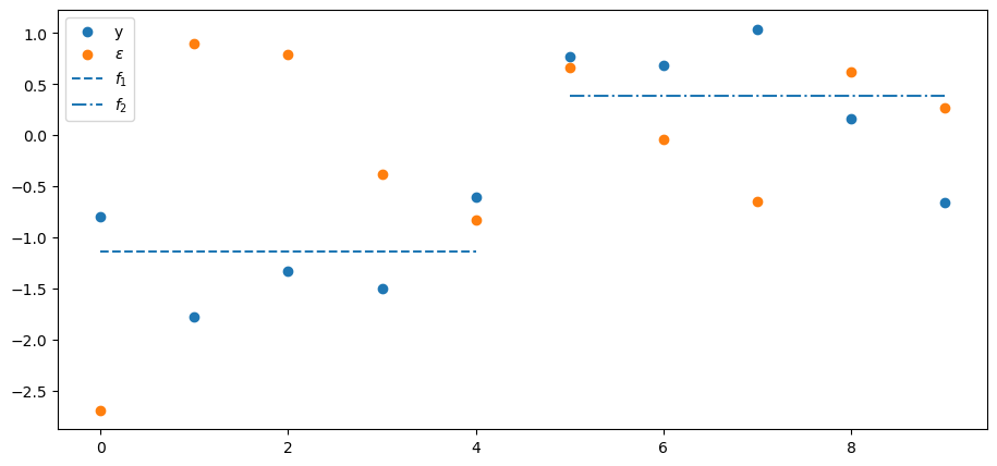
_images/655ab11cf4def6a8e2cf53731712757091c3f353edbc0453557861bc06034901.png

Consequently, the first two $ϵ_{j}$ correspond to the largest two eigenvalues.

Let’s look at them, after which we’ll look at $E f | y = B y$

ε[:2]

array([-2.68965844,  0.89427629])

# compare with Ef|y
B @ y

array([-1.14557316,  0.38088811])

The fraction of variance in $y_{t}$ explained by the first two principal components can be computed as below.

𝜆_tilde[:2].sum() / 𝜆_tilde.sum()

0.84

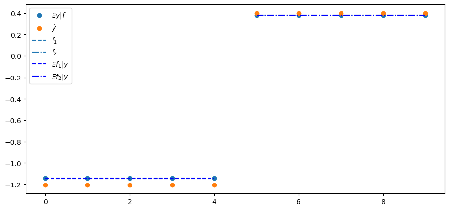
Compute

\hat{Y} = P_{j} ϵ_{j} + P_{k} ϵ_{k}

where $P_{j}$ and $P_{k}$ correspond to the largest two eigenvalues.

y_hat = P[:, :2] @ ε[:2]

In this example, it turns out that the projection $\hat{Y}$ of $Y$ on the first two principal components does a good job of approximating $E f ∣ y$ .

We confirm this in the following plot of $f$ , $E y ∣ f$ , $E f ∣ y$ , and $\hat{y}$ on the coordinate axis versus $y$ on the ordinate axis.

plt.scatter(range(N), Λ @ f, label='$Ey|f$')
plt.scatter(range(N), y_hat, label=r'$\hat{y}$')
plt.hlines(f[0], 0, N//2-1, ls='--', label='$f_{1}$')
plt.hlines(f[1], N//2, N-1, ls='-.', label='$f_{2}$')

Efy = B @ y
plt.hlines(Efy[0], 0, N//2-1, ls='--', color='b', label='$Ef_{1}|y$')
plt.hlines(Efy[1], N//2, N-1, ls='-.', color='b', label='$Ef_{2}|y$')
plt.legend()

plt.show()

_images/a6865405d0337461ab6e4aeadaaeac0dce27e18fc69f2a2c307cb4d68c769413.png

The covariance matrix of $\hat{Y}$ can be computed by first constructing the covariance matrix of $ϵ$ and then use the upper left block for $ϵ_{1}$ and $ϵ_{2}$ .

Σεjk = (P.T @ Σy @ P)[:2, :2]

Pjk = P[:, :2]

Σy_hat = Pjk @ Σεjk @ Pjk.T
print('Σy_hat = \n', Σy_hat)

Σy_hat = 
 [[1.05 1.05 1.05 1.05 1.05 0.   0.   0.   0.   0.  ]
 [1.05 1.05 1.05 1.05 1.05 0.   0.   0.   0.   0.  ]
 [1.05 1.05 1.05 1.05 1.05 0.   0.   0.   0.   0.  ]
 [1.05 1.05 1.05 1.05 1.05 0.   0.   0.   0.   0.  ]
 [1.05 1.05 1.05 1.05 1.05 0.   0.   0.   0.   0.  ]
 [0.   0.   0.   0.   0.   1.05 1.05 1.05 1.05 1.05]
 [0.   0.   0.   0.   0.   1.05 1.05 1.05 1.05 1.05]
 [0.   0.   0.   0.   0.   1.05 1.05 1.05 1.05 1.05]
 [0.   0.   0.   0.   0.   1.05 1.05 1.05 1.05 1.05]
 [0.   0.   0.   0.   0.   1.05 1.05 1.05 1.05 1.05]]